Plot Stepleman & Winarsky's method

Find a step which is near to optimal for a central finite difference formula.

References

• Adaptive numerical differentiation R. S. Stepleman and N. D. Winarsky Journal: Math. Comp. 33 (1979), 1257-1264

import numpy as np
import pylab as pl
import tabulate
import numericalderivative as nd

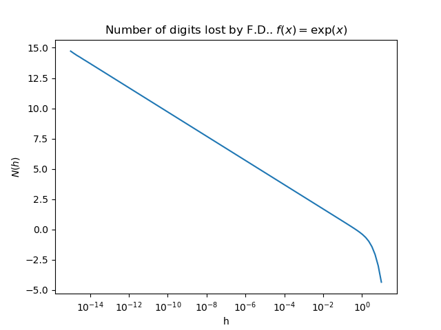
Plot the number of lost digits for exp

number_of_points = 100
x = 1.0
step_array = np.logspace(-15.0, 1.0, number_of_points)
n_digits_array = np.zeros((number_of_points))
algorithm = nd.SteplemanWinarsky(np.exp, x)
initialize = nd.SteplemanWinarskyInitialize(algorithm)
for i in range(number_of_points):
    h = step_array[i]
    n_digits_array[i] = initialize.number_of_lost_digits(h)

pl.figure()
pl.plot(step_array, n_digits_array)
pl.title(r"Number of digits lost by F.D.. $f(x) = \exp(x)$")
pl.xlabel("h")
pl.ylabel("$N(h)$")
pl.xscale("log")

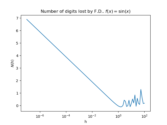
Plot the number of lost digits for sin

x = 1.0
step_array = np.logspace(-7.0, 2.0, number_of_points)
n_digits_array = np.zeros((number_of_points))
algorithm = nd.SteplemanWinarsky(np.sin, x)
initialize = nd.SteplemanWinarskyInitialize(algorithm)
for i in range(number_of_points):
    h = step_array[i]
    n_digits_array[i] = initialize.number_of_lost_digits(h)

pl.figure()
pl.plot(step_array, n_digits_array)
pl.title(r"Number of digits lost by F.D.. $f(x) = \sin(x)$")
pl.xlabel("h")
pl.ylabel("$N(h)$")
pl.xscale("log")

For each function, at point x = 1, plot the error vs the step computed by the method

def plot_error_vs_h_with_SW_steps(
    name, function, function_derivative, x, step_array, h_min, h_max, verbose=False
):
    """
    Plot the computed error depending on the step for an array of F.D. steps

    Parameters
    ----------
    name : str
        The name of the problem
    function : function
        The function.
    first_derivative : function
        The exact first derivative of the function
    x : float
        The input point where the test is done
    step_array : list(float)
        The array of finite difference steps
    h_min : float, > 0
        The lower bound to bracket the initial differentiation step.
    h_max : float, > kmin
        The upper bound to bracket the initial differentiation step.
    verbose : bool, optional
        Set to True to print intermediate messages. The default is False.
    """
    algorithm = nd.SteplemanWinarsky(function, x)
    initialize = nd.SteplemanWinarskyInitialize(algorithm)
    number_of_points = len(step_array)
    error_array = np.zeros((number_of_points))
    for i in range(number_of_points):
        h = step_array[i]
        f_prime_approx = algorithm.compute_first_derivative(h)
        error_array[i] = abs(f_prime_approx - function_derivative(x))

    bisection_h0_step, bisection_h0_iteration = initialize.find_initial_step(
        h_min, h_max
    )
    step, bisection_iterations = algorithm.find_step(bisection_h0_step)

    if verbose:
        print(name)
        print(f"h_min = {h_min:.3e}, h_max = {h_max:.3e}")
        print(
            "Bisection initial_step = %.3e using %d iterations"
            % (bisection_h0_step, bisection_h0_iteration)
        )
        print("Bisection h* = %.3e using %d iterations" % (step, bisection_iterations))

    minimum_error = np.nanmin(error_array)
    maximum_error = np.nanmax(error_array)

    pl.figure()
    pl.plot(step_array, error_array)
    pl.plot(
        [h_min] * 2,
        [minimum_error, maximum_error],
        "--",
        label=r"$h_{\min}$",
    )
    pl.plot(
        [h_max] * 2,
        [minimum_error, maximum_error],
        "--",
        label=r"$h_{\max}$",
    )
    pl.plot(
        [bisection_h0_step] * 2,
        [minimum_error, maximum_error],
        "--",
        label="$h_{0}^{(B)}$",
    )
    pl.plot([step] * 2, [minimum_error, maximum_error], "--", label="$h^{*}$")
    pl.title("Finite difference : %s at point x = %.0f" % (name, x))
    pl.xlabel("h")
    pl.ylabel("Error")
    pl.xscale("log")
    pl.yscale("log")
    pl.legend(bbox_to_anchor=(1.0, 1.0))
    pl.subplots_adjust(right=0.8)
    return

def plot_error_vs_h_benchmark(problem, x, step_array, h_min, h_max, verbose=False):
    """
    Plot the computed error depending on the step for an array of F.D. steps

    Parameters
    ----------
    problem : nd.BenchmarkProblem
        The problem
    x : float
        The input point where the test is done
    step_array : list(float)
        The array of finite difference steps
    kmin : float, > 0
        The minimum step k for the second derivative.
    kmax : float, > kmin
        The maximum step k for the second derivative.
    verbose : bool, optional
        Set to True to print intermediate messages. The default is False.
    """
    plot_error_vs_h_with_SW_steps(
        problem.get_name(),
        problem.get_function(),
        problem.get_first_derivative(),
        x,
        step_array,
        h_min,
        h_max,
        True,
    )

problem = nd.ExponentialProblem()
x = 1.0
number_of_points = 1000
step_array = np.logspace(-15.0, 1.0, number_of_points)
plot_error_vs_h_benchmark(problem, x, step_array, 1.0e-10, 1.0e0, True)

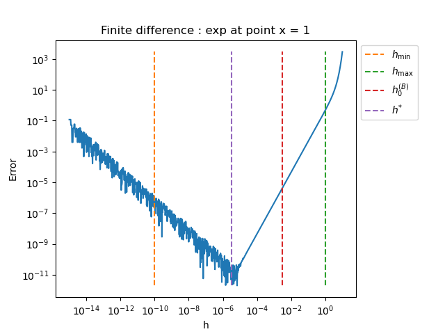
exp
h_min = 1.000e-10, h_max = 1.000e+00
Bisection initial_step = 3.162e-03 using 1 iterations
Bisection h* = 3.088e-06 using 5 iterations

x = 12.0
step_array = np.logspace(-15.0, 1.0, number_of_points)
plot_error_vs_h_benchmark(problem, x, step_array, 1.0e-10, 1.0e0)

if False:
    problem = nd.LogarithmicProblem()
    x = 1.0
    plot_error_vs_h_benchmark(problem, x, step_array, 1.0e-15, 1.0e0, True)

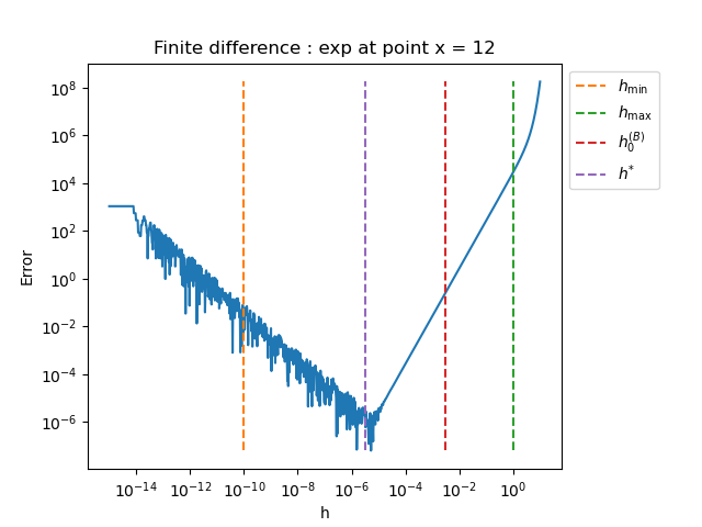
exp
h_min = 1.000e-10, h_max = 1.000e+00
Bisection initial_step = 3.162e-03 using 1 iterations
Bisection h* = 3.088e-06 using 5 iterations

problem = nd.LogarithmicProblem()
x = 1.1
step_array = np.logspace(-15.0, -1.0, number_of_points)
plot_error_vs_h_benchmark(problem, x, step_array, 1.0e-14, 1.0e-1, True)

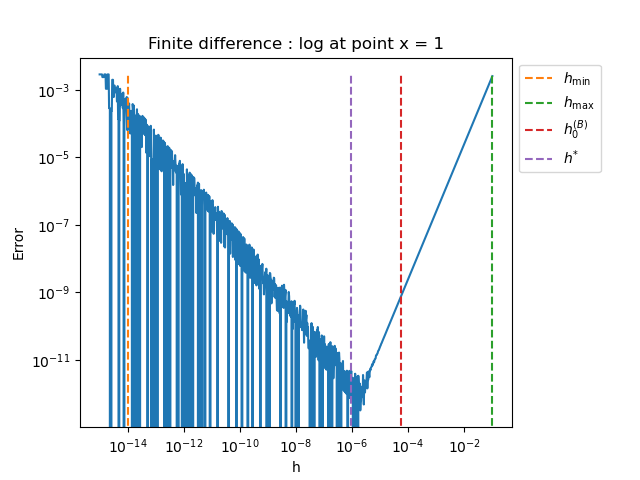
log
h_min = 1.000e-14, h_max = 1.000e-01
Bisection initial_step = 5.623e-05 using 1 iterations
Bisection h* = 8.787e-07 using 3 iterations

problem = nd.SinProblem()
x = 1.0
step_array = np.logspace(-15.0, 0.0, number_of_points)
plot_error_vs_h_benchmark(problem, x, step_array, 1.0e-15, 1.0e-0)

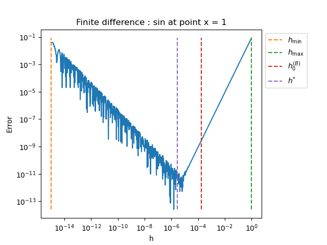
sin
h_min = 1.000e-15, h_max = 1.000e+00
Bisection initial_step = 1.778e-04 using 1 iterations
Bisection h* = 2.779e-06 using 3 iterations

problem = nd.SquareRootProblem()
x = 1.0
step_array = np.logspace(-15.0, 0.0, number_of_points)
plot_error_vs_h_benchmark(problem, x, step_array, 1.0e-15, 1.0e-0, True)

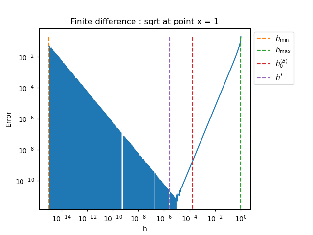
sqrt
h_min = 1.000e-15, h_max = 1.000e+00
Bisection initial_step = 1.778e-04 using 1 iterations
Bisection h* = 2.779e-06 using 3 iterations

problem = nd.AtanProblem()
x = 1.0
step_array = np.logspace(-15.0, 0.0, number_of_points)
plot_error_vs_h_benchmark(problem, x, step_array, 1.0e-15, 1.0e-0)

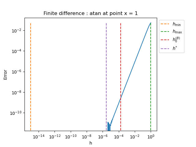
atan
h_min = 1.000e-15, h_max = 1.000e+00
Bisection initial_step = 1.778e-04 using 1 iterations
Bisection h* = 2.779e-06 using 3 iterations

problem = nd.ExponentialProblem()
print("+ Sensitivity of SW step depending on initial_step")
print("Case 1 : exp")
x = 1.0
function = problem.get_function()
third_derivative = problem.get_third_derivative()
algorithm = nd.SteplemanWinarsky(
    function,
    x,
)
third_derivative_value = third_derivative(x)
optimal_step, absolute_error = nd.FirstDerivativeCentral.compute_step(
    third_derivative_value
)
print("Exact h* = %.3e" % (optimal_step))
print("absolute_error = %.3e" % (absolute_error))
for initial_step in np.logspace(-4, 0, 10):
    estim_step, iterations = algorithm.find_step(initial_step)
    print(
        "initial_step = %.3e, Approx. h* = %.3e (%d iterations)"
        % (initial_step, estim_step, iterations)
    )

print("Case 2 : Scaled exp")
x = 1.0

+ Sensitivity of SW step depending on initial_step
Case 1 : exp
Exact h* = 4.797e-06
absolute_error = 3.127e-11
initial_step = 1.000e-04, Approx. h* = 1.563e-06 (3 iterations)
initial_step = 2.783e-04, Approx. h* = 1.087e-06 (4 iterations)
initial_step = 7.743e-04, Approx. h* = 3.024e-06 (4 iterations)
initial_step = 2.154e-03, Approx. h* = 2.104e-06 (5 iterations)
initial_step = 5.995e-03, Approx. h* = 5.854e-06 (5 iterations)
initial_step = 1.668e-02, Approx. h* = 1.018e-06 (7 iterations)
initial_step = 4.642e-02, Approx. h* = 2.833e-06 (7 iterations)
initial_step = 1.292e-01, Approx. h* = 1.971e-06 (8 iterations)
initial_step = 3.594e-01, Approx. h* = 1.371e-06 (9 iterations)
initial_step = 1.000e+00, Approx. h* = 9.537e-07 (10 iterations)
Case 2 : Scaled exp

problem = nd.ScaledExponentialProblem()
function = problem.get_function()
third_derivative = problem.get_third_derivative()
x = problem.get_x()
algorithm = nd.SteplemanWinarsky(function, x)
third_derivative_value = third_derivative(x)
optimal_step, absolute_error = nd.FirstDerivativeCentral.compute_step(
    third_derivative_value
)
print("Exact h* = %.3e" % (optimal_step))
print("absolute_error = %.3e" % (absolute_error))
for initial_step in np.logspace(0, 6, 10):
    estim_step, iterations = algorithm.find_step(initial_step)
    print(
        "initial_step = %.3e, Approx. h* = %.3e (%d iterations)"
        % (initial_step, estim_step, iterations)
    )

Exact h* = 6.694e+00
absolute_error = 2.241e-17
initial_step = 1.000e+00, Approx. h* = 2.500e-01 (1 iterations)
initial_step = 4.642e+00, Approx. h* = 1.160e+00 (1 iterations)
initial_step = 2.154e+01, Approx. h* = 1.347e+00 (2 iterations)
initial_step = 1.000e+02, Approx. h* = 1.562e+00 (3 iterations)
initial_step = 4.642e+02, Approx. h* = 1.813e+00 (4 iterations)
initial_step = 2.154e+03, Approx. h* = 8.416e+00 (4 iterations)
initial_step = 1.000e+04, Approx. h* = 2.441e+00 (6 iterations)
initial_step = 4.642e+04, Approx. h* = 2.833e+00 (7 iterations)
initial_step = 2.154e+05, Approx. h* = 3.287e+00 (8 iterations)
initial_step = 1.000e+06, Approx. h* = 3.815e+00 (9 iterations)