Use the finite differences formulas

This example shows how to use finite difference (F.D.) formulas.

References

• 13. Baudin (2023). Méthodes numériques. Dunod.

import numericalderivative as nd
import numpy as np
import pylab as pl

Compute the first derivative using forward F.D. formula

This is the function we want to compute the derivative of.

def scaled_exp(x):
    alpha = 1.0e6
    return np.exp(-x / alpha)

Use the F.D. formula

x = 1.0
finite_difference = nd.FirstDerivativeForward(scaled_exp, x)
step = 1.0e-3  # A first guess
f_prime_approx = finite_difference.compute(step)
print(f"Approximate f'(x) = {f_prime_approx}")

Approximate f'(x) = -9.999989725174565e-07

To check our result, we define the exact first derivative.

def scaled_exp_prime(x):
    alpha = 1.0e6
    return -np.exp(-x / alpha) / alpha

Compute the exact derivative and the absolute error.

f_prime_exact = scaled_exp_prime(x)
print(f"Exact f'(x) = {f_prime_exact}")
absolute_error = abs(f_prime_approx - f_prime_exact)
print(f"Absolute error = {absolute_error}")

Exact f'(x) = -9.999990000005e-07
Absolute error = 2.748304361188279e-14

Define the error function: this will be useful later.

def compute_absolute_error(step, x=1.0, verbose=True):
    finite_difference = nd.FirstDerivativeForward(scaled_exp, x)
    f_prime_approx = finite_difference.compute(step)
    f_prime_exact = scaled_exp_prime(x)
    absolute_error = abs(f_prime_approx - f_prime_exact)
    if verbose:
        print(f"Approximate f'(x) = {f_prime_approx}")
        print(f"Exact f'(x) = {f_prime_exact}")
        print(f"Absolute error = {absolute_error}")
    return absolute_error

Compute the exact step for the forward F.D. formula

This step depends on the second derivative. Firstly, we assume that this is unknown and use a first guess of it, equal to 1.

second_derivative_value = 1.0
step, absolute_error = nd.FirstDerivativeForward.compute_step(second_derivative_value)
print(f"Approximately optimal step (using f''(x) = 1) = {step}")
print(f"Approximately absolute error = {absolute_error}")
_ = compute_absolute_error(step, True)

Approximately optimal step (using f''(x) = 1) = 2e-08
Approximately absolute error = 2e-08
Approximate f'(x) = -9.992007171418978e-07
Exact f'(x) = -9.999990000005e-07
Absolute error = 7.982828586023276e-10

We see that the new step is much better than the our initial guess: the approximately optimal step is much smaller, which leads to a smaller absolute error.

In our particular example, the second derivative is known: let's use this information and compute the exactly optimal step.

def scaled_exp_2nd_derivative(x):
    alpha = 1.0e6
    return np.exp(-x / alpha) / (alpha**2)

second_derivative_value = scaled_exp_2nd_derivative(x)
print(f"Exact second derivative f''(x) = {second_derivative_value}")
step, absolute_error = nd.FirstDerivativeForward.compute_step(second_derivative_value)
print(f"Approximately optimal step (using f''(x) = 1) = {step}")
print(f"Approximately absolute error = {absolute_error}")
_ = compute_absolute_error(step, True)

Exact second derivative f''(x) = 9.999990000005e-13
Approximately optimal step (using f''(x) = 1) = 0.0200000100000025
Approximately absolute error = 1.99999900000025e-14
Approximate f'(x) = -9.999989887714385e-07
Exact f'(x) = -9.999990000005e-07
Absolute error = 1.1229061571641635e-14

def plot_step_sensitivity(
    finite_difference,
    x,
    function_derivative,
    step_array,
    higher_derivative_value,
    relative_error=1.0e-16,
):
    """
    Compute the approximate derivative using central F.D. formula.
    Create a plot representing the absolute error depending on step.

    Parameters
    ----------
    finite_difference : FiniteDifferenceFormula
        The F.D. formula
    x : float
        The input point
    function_derivative : function
        The exact derivative of the function.
    step_array : array(n_points)
        The array of steps to consider
    higher_derivative_value : float
        The value of the higher derivative required for the optimal step for the derivative
    """
    number_of_points = len(step_array)
    error_array = np.zeros((number_of_points))
    for i in range(number_of_points):
        f_prime_approx = finite_difference.compute(step_array[i])
        error_array[i] = abs(f_prime_approx - function_derivative(x))

    pl.figure()
    pl.plot(step_array, error_array, label="Computed")
    pl.title(finite_difference.__class__.__name__)
    pl.xlabel("h")
    pl.ylabel("Error")
    pl.xscale("log")
    pl.legend(bbox_to_anchor=(1.0, 1.0))
    pl.yscale("log")

    # Compute the error using the model
    function = finite_difference.get_function().get_function()
    absolute_precision_function_eval = abs(function(x)) * relative_error
    error_array = np.zeros((number_of_points))
    for i in range(number_of_points):
        error_array[i] = finite_difference.compute_error(
            step_array[i], higher_derivative_value, absolute_precision_function_eval
        )

    pl.plot(step_array, error_array, "--", label="Model")
    # Compute the optimal step size and optimal error
    optimal_step, absolute_error = finite_difference.compute_step(
        higher_derivative_value, absolute_precision_function_eval
    )
    pl.plot([optimal_step], [absolute_error], "o", label=r"$(h^*, e(h^*))$")
    #
    pl.tight_layout()
    return

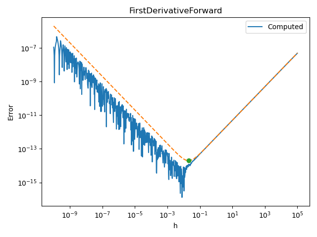
For the forward F.D. formula, the absolute error is known if the second derivative value can be computed. The next script uses this feature from the compute_error() method to plot the upper bound of the error.

number_of_points = 1000
step_array = np.logspace(-10.0, 5.0, number_of_points)
finite_difference = nd.FirstDerivativeForward(scaled_exp, x)
plot_step_sensitivity(
    finite_difference, x, scaled_exp_prime, step_array, second_derivative_value
)

These features are available with most F.D. formulas: the next sections show how the module provides the exact optimal step and the exact error for other formulas.

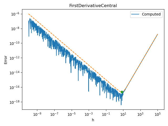
Central F.D. formula for first derivative

Let us see how this behaves with central F.D.

# For the central F.D. formula, the exact step depends on the
# third derivative
def scaled_exp_3d_derivative(x):
    alpha = 1.0e6
    return -np.exp(-x / alpha) / (alpha**3)

number_of_points = 1000
step_array = np.logspace(-10.0, 5.0, number_of_points)
finite_difference = nd.FirstDerivativeCentral(scaled_exp, x)
third_derivative_value = scaled_exp_3d_derivative(x)
plot_step_sensitivity(
    finite_difference, x, scaled_exp_prime, step_array, third_derivative_value
)

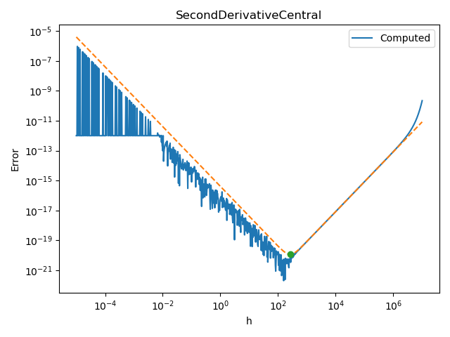
Central F.D. formula for second derivative

Let us see how this behaves with central F.D. for the second derivative.

For the central F.D. formula of the second derivative, the exact step depends on the fourth derivative

def scaled_exp_4th_derivative(x):
    alpha = 1.0e6
    return np.exp(-x / alpha) / (alpha**4)

number_of_points = 1000
step_array = np.logspace(-5.0, 7.0, number_of_points)
finite_difference = nd.SecondDerivativeCentral(scaled_exp, x)
fourth_derivative_value = scaled_exp_4th_derivative(x)
plot_step_sensitivity(
    finite_difference, x, scaled_exp_2nd_derivative, step_array, fourth_derivative_value
)

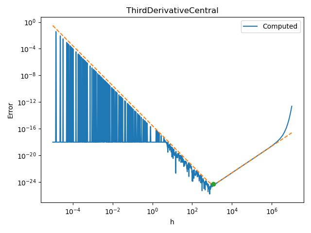
Central F.D. formula for third derivative

Let us see how this behaves with central F.D. for the third derivative.

For the central F.D. formula of the third derivative, the exact step depends on the fifth derivative

def scaled_exp_5th_derivative(x):
    alpha = 1.0e6
    return np.exp(-x / alpha) / (alpha**5)

number_of_points = 1000
step_array = np.logspace(-5.0, 7.0, number_of_points)
finite_difference = nd.ThirdDerivativeCentral(scaled_exp, x)
fifth_derivative_value = scaled_exp_5th_derivative(x)
plot_step_sensitivity(
    finite_difference, x, scaled_exp_3d_derivative, step_array, fifth_derivative_value
)