Use the benchmark problems

This example shows how to use a single benchmark problem or all the problems.

import tabulate
import numericalderivative as nd
import math
import pylab as pl
import numpy as np

First, we create an use a single problem. We create the problem and get the function and its first derivative. Printing the object evaluates the function and its derivatives at the test point.

problem = nd.ExponentialProblem()
print(problem)

DerivativeBenchmarkProblem
name = exp
x = 1.0
f(x) = 2.718281828459045
f'(x) = 2.718281828459045
f''(x) = 2.718281828459045
f^(3)(x) = 2.718281828459045
f^(4)(x) = 2.718281828459045
f^(5)(x) = 2.718281828459045

We can also use the pretty-print.

problem

DerivativeBenchmarkProblem

• name = exp
• x = 1.0
• f(x) = 2.718281828459045
• f'(x) = 2.718281828459045
• f''(x) = 2.718281828459045
• f^(3)(x) = 2.718281828459045
• f^(4)(x) = 2.718281828459045
• f^(5)(x) = 2.718281828459045

Get the data from the problem

x = problem.get_x()
function = problem.get_function()
first_derivative = problem.get_first_derivative()

Then we use a finite difference formula and compare it to the exact derivative.

formula = nd.FirstDerivativeForward(function, x)
step = 1.0e-5  # This is a first guess
approx_first_derivative = formula.compute(step)
exact_first_derivative = first_derivative(x)
absolute_error = abs(approx_first_derivative - exact_first_derivative)
print(f"Approximate first derivative = {approx_first_derivative}")
print(f"Exact first derivative = {exact_first_derivative}")
print(f"Absolute error = {absolute_error}")

Approximate first derivative = 2.7182954199389098
Exact first derivative = 2.718281828459045
Absolute error = 1.359147986468301e-05

The problem is that the optimal step might not be the exact one. The optimal step can be computed using the second derivative, which is known in this problem.

second_derivative = problem.get_second_derivative()
second_derivative_value = second_derivative(x)
optimal_step_forward_formula, absolute_error = nd.FirstDerivativeForward.compute_step(
    second_derivative_value
)
print(f"Optimal step for forward derivative = {optimal_step_forward_formula}")
print(f"Minimum absolute error = {absolute_error}")

Optimal step for forward derivative = 1.2130613194252668e-08
Minimum absolute error = 3.297442541400256e-08

Now use this step

approx_first_derivative = formula.compute(optimal_step_forward_formula)
exact_first_derivative = first_derivative(x)
absolute_error = abs(approx_first_derivative - exact_first_derivative)
print(f"Approximate first derivative = {approx_first_derivative}")
print(f"Exact first derivative = {exact_first_derivative}")
print(f"Absolute error = {absolute_error}")

Approximate first derivative = 2.718281867990813
Exact first derivative = 2.718281828459045
Absolute error = 3.953176808124681e-08

We can use a collection of benchmark problems.

benchmark = nd.build_benchmark()
number_of_problems = len(benchmark)
data = []
for i in range(number_of_problems):
    problem = benchmark[i]
    name = problem.get_name()
    x = problem.get_x()
    interval = problem.get_interval()
    data.append(
        [
            f"#{i} / {number_of_problems}",
            f"{name}",
            f"{x}",
            f"{interval[0]}",
            f"{interval[1]}",
        ]
    )

tabulate.tabulate(
    data,
    headers=["Index", "Name", "x", "xmin", "xmax"],
    tablefmt="html",
)

Index	Name	x	xmin	xmax
#0 / 16	polynomial	1	-12	12
#1 / 16	inverse	1	0.01	12
#2 / 16	exp	1	0	12
#3 / 16	log	1	0.01	12
#4 / 16	sqrt	1	0.01	12
#5 / 16	atan	0.5	-12	12
#6 / 16	sin	1	-3.14159	3.14159
#7 / 16	scaled exp	1	0	12
#8 / 16	GMSW	1	0.001	12
#9 / 16	SXXN1	-8	-12	12
#10 / 16	SXXN2	0.01	-1	1
#11 / 16	SXXN3	0.99999	-12	12
#12 / 16	SXXN4	1e-09	-12	12
#13 / 16	Oliver1	1	-12	12
#14 / 16	Oliver2	1	-12	12
#15 / 16	Oliver3	1	0.01	12

Print each benchmark problems.

benchmark = nd.build_benchmark()
number_of_problems = len(benchmark)
for i in range(number_of_problems):
    problem = benchmark[i]
    print(problem)

DerivativeBenchmarkProblem
name = polynomial
x = 1.0
f(x) = 1.0
f'(x) = 2.0
f''(x) = 2.0
f^(3)(x) = 0.0
f^(4)(x) = 0.0
f^(5)(x) = 0.0

DerivativeBenchmarkProblem
name = inverse
x = 1.0
f(x) = 1.0
f'(x) = -1.0
f''(x) = 2.0
f^(3)(x) = -6.0
f^(4)(x) = 24.0
f^(5)(x) = -120.0

DerivativeBenchmarkProblem
name = exp
x = 1.0
f(x) = 2.718281828459045
f'(x) = 2.718281828459045
f''(x) = 2.718281828459045
f^(3)(x) = 2.718281828459045
f^(4)(x) = 2.718281828459045
f^(5)(x) = 2.718281828459045

DerivativeBenchmarkProblem
name = log
x = 1.0
f(x) = 0.0
f'(x) = 1.0
f''(x) = -1.0
f^(3)(x) = 2.0
f^(4)(x) = -6.0
f^(5)(x) = 24.0

DerivativeBenchmarkProblem
name = sqrt
x = 1.0
f(x) = 1.0
f'(x) = 0.5
f''(x) = -0.25
f^(3)(x) = 0.375
f^(4)(x) = -0.9375
f^(5)(x) = 3.28125

DerivativeBenchmarkProblem
name = atan
x = 0.5
f(x) = 0.4636476090008061
f'(x) = 0.8
f''(x) = -0.64
f^(3)(x) = -0.256
f^(4)(x) = 3.6864
f^(5)(x) = -9.33888

DerivativeBenchmarkProblem
name = sin
x = 1.0
f(x) = 0.8414709848078965
f'(x) = 0.5403023058681398
f''(x) = -0.8414709848078965
f^(3)(x) = -0.5403023058681398
f^(4)(x) = 0.8414709848078965
f^(5)(x) = 0.5403023058681398

DerivativeBenchmarkProblem
name = scaled exp
x = 1.0
f(x) = 0.9999990000005
f'(x) = -9.999990000004999e-07
f''(x) = 9.999990000005e-13
f^(3)(x) = -9.999990000005e-19
f^(4)(x) = 9.999990000004998e-25
f^(5)(x) = -9.999990000004998e-31

DerivativeBenchmarkProblem
name = GMSW
x = 1.0
f(x) = 3.0382788796394644
f'(x) = 9.548655322129756
f''(x) = 24.266107348211236
f^(3)(x) = 53.1455550486372
f^(4)(x) = 113.23547948425671
f^(5)(x) = 211.44420430021552

DerivativeBenchmarkProblem
name = SXXN1
x = -8.0
f(x) = 0.9993291872793697
f'(x) = -0.0006707001854555852
f''(x) = -0.0006704751151061466
f^(3)(x) = -0.0006700249744072696
f^(4)(x) = -0.0006691246930095155
f^(5)(x) = -0.0006673241302140074

DerivativeBenchmarkProblem
name = SXXN2
x = 0.01
f(x) = 2.718281828459045
f'(x) = 271.8281828459045
f''(x) = 27182.818284590452
f^(3)(x) = 2718281.828459045
f^(4)(x) = 271828182.8459045
f^(5)(x) = 27182818284.59045

DerivativeBenchmarkProblem
name = SXXN3
x = 0.99999
f(x) = -5.9999999991000035
f'(x) = -0.00017999880000374446
f''(x) = 17.999760001200002
f^(3)(x) = 23.999760000000002
f^(4)(x) = 24
f^(5)(x) = 0.0

DerivativeBenchmarkProblem
name = SXXN4
x = 1e-09
f(x) = 5.00000000001001e-09
f'(x) = 5.00000000002003
f''(x) = 0.02006
f^(3)(x) = 60000.0
f^(4)(x) = 0
f^(5)(x) = 0

DerivativeBenchmarkProblem
name = Oliver1
x = 1.0
f(x) = 54.598150033144236
f'(x) = 218.39260013257694
f''(x) = 873.5704005303078
f^(3)(x) = 3494.281602121231
f^(4)(x) = 13977.126408484924
f^(5)(x) = 55908.5056339397

DerivativeBenchmarkProblem
name = Oliver2
x = 1.0
f(x) = 2.718281828459045
f'(x) = 5.43656365691809
f''(x) = 16.30969097075427
f^(3)(x) = 54.3656365691809
f^(4)(x) = 206.58941896288744
f^(5)(x) = 848.1039304792221

DerivativeBenchmarkProblem
name = Oliver3
x = 1.0
f(x) = 0.0
f'(x) = 1.0
f''(x) = 3.0
f^(3)(x) = 2.0
f^(4)(x) = -2.0
f^(5)(x) = 4.0

Plot the benchmark problems.

benchmark = nd.build_benchmark()
number_of_problems = len(benchmark)
number_of_columns = 3
number_of_rows = math.ceil(number_of_problems / number_of_columns)
number_of_points = 100
pl.figure(figsize=(8.0, 7.0))
data = []
index = 1
for i in range(number_of_problems):
    problem = benchmark[i]
    name = problem.get_name()
    print(f"Plot #{i}: {name}")
    x = problem.get_x()
    interval = problem.get_interval()
    function = problem.get_function()
    pl.subplot(number_of_rows, number_of_columns, index)
    x_grid = np.linspace(interval[0], interval[1], number_of_points)
    y_values = function(x_grid)
    pl.title(f"{name}")
    pl.plot(x_grid, y_values)
    # Update index
    index += 1

pl.subplots_adjust(wspace=0.5, hspace=1.2)

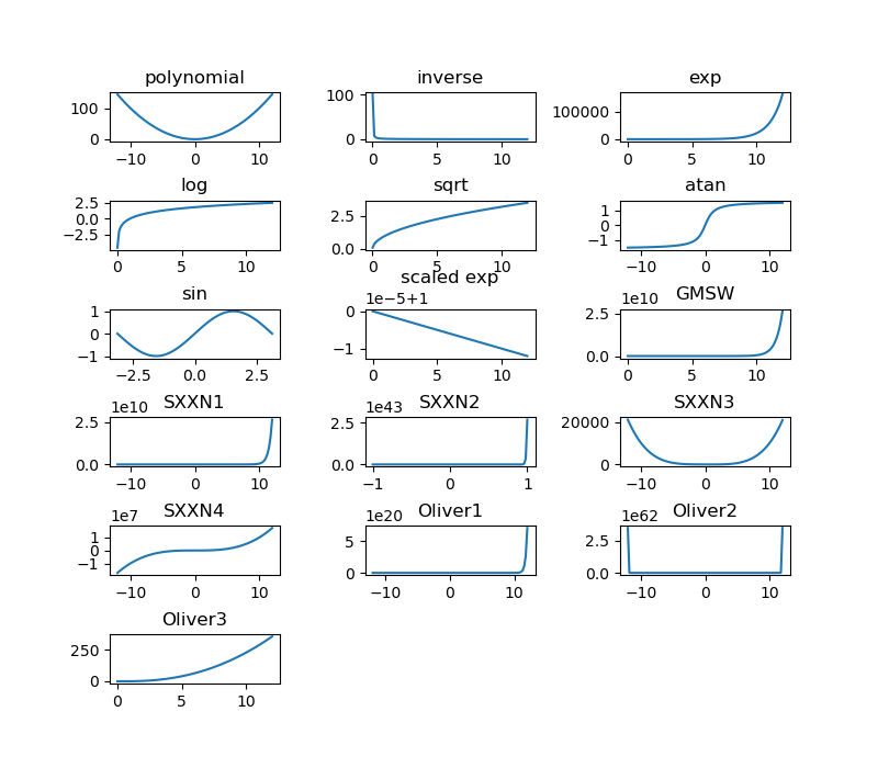
Plot #0: polynomial
Plot #1: inverse
Plot #2: exp
Plot #3: log
Plot #4: sqrt
Plot #5: atan
Plot #6: sin
Plot #7: scaled exp
Plot #8: GMSW
Plot #9: SXXN1
Plot #10: SXXN2
Plot #11: SXXN3
Plot #12: SXXN4
Plot #13: Oliver1
Plot #14: Oliver2
Plot #15: Oliver3