Note
Go to the end to download the full example code.
Use the generalized finite differences formulas
This example shows how to use generalized finite difference (F.D.) formulas.
References
Baudin (2023). Méthodes numériques. Dunod.
import numericalderivative as nd
import numpy as np
import pylab as pl
import matplotlib.colors as mcolors
import tabulate
Compute the first derivative using forward F.D. formula
This is the function we want to compute the derivative of.
def scaled_exp(x):
    alpha = 1.0e6
    return np.exp(-x / alpha)
Use the F.D. formula for f'(x)
x = 1.0
differentiation_order = 1
formula_accuracy = 2
finite_difference = nd.GeneralFiniteDifference(
    scaled_exp, x, differentiation_order, formula_accuracy, "central"
)
step = 1.0e-3  # A first guess
f_prime_approx = finite_difference.compute(step)
print(f"Approximate f'(x) = {f_prime_approx}")
Approximate f'(x) = -9.999989725173464e-07
To check our result, we define the exact first derivative.
def scaled_exp_prime(x):
    alpha = 1.0e6
    return -np.exp(-x / alpha) / alpha
Compute the exact derivative and the absolute error.
f_prime_exact = scaled_exp_prime(x)
print(f"Exact f'(x) = {f_prime_exact}")
absolute_error = abs(f_prime_approx - f_prime_exact)
print(f"Absolute error = {absolute_error}")
Exact f'(x) = -9.999990000005e-07
Absolute error = 2.7483153726165933e-14
Define the error function: this will be useful later.
def compute_absolute_error(
    step,
    x=1.0,
    differentiation_order=1,
    formula_accuracy=2,
    direction="central",
    verbose=True,
):
    finite_difference = nd.GeneralFiniteDifference(
        scaled_exp, x, differentiation_order, formula_accuracy, direction
    )
    f_prime_approx = finite_difference.compute(step)
    f_prime_exact = scaled_exp_prime(x)
    absolute_error = abs(f_prime_approx - f_prime_exact)
    if verbose:
        print(f"Approximate f'(x) = {f_prime_approx}")
        print(f"Exact f'(x) = {f_prime_exact}")
        print(f"Absolute error = {absolute_error}")
    return absolute_error
Compute the exact step for the forward F.D. formula
This step depends on the second derivative. Firstly, we assume that this is unknown and use a first guess of it, equal to 1.
differentiation_order = 1
formula_accuracy = 2
direction = "central"
finite_difference = nd.GeneralFiniteDifference(
    scaled_exp, x, differentiation_order, formula_accuracy, direction
)
second_derivative_value = 1.0  # A first guess
step, absolute_error = finite_difference.compute_step(second_derivative_value)
print(f"Approximately optimal step (using f''(x) = 1) = {step}")
print(f"Approximately absolute error = {absolute_error}")
_ = compute_absolute_error(step, True)
Approximately optimal step (using f''(x) = 1) = 8.733476581980381e-06
Approximately absolute error = 3.8136806603999814e-11
Approximate f'(x) = -9.999979182323467e-07
Exact f'(x) = -9.999990000005e-07
Absolute error = 1.081768153431351e-12
We see that the new step is much better than the our initial guess: the approximately optimal step is much smaller, which leads to a smaller absolute error.
In our particular example, the second derivative is known: let's use this information and compute the exactly optimal step.
def scaled_exp_2nd_derivative(x):
    alpha = 1.0e6
    return np.exp(-x / alpha) / (alpha**2)
second_derivative_value = scaled_exp_2nd_derivative(x)
print(f"Exact second derivative f''(x) = {second_derivative_value}")
step, absolute_error = finite_difference.compute_step(second_derivative_value)
print(f"Approximately optimal step (using f''(x) = 1) = {step}")
print(f"Approximately absolute error = {absolute_error}")
_ = compute_absolute_error(step, True)
Exact second derivative f''(x) = 9.999990000005e-13
Approximately optimal step (using f''(x) = 1) = 0.08733479493139723
Approximately absolute error = 3.813679389173307e-15
Approximate f'(x) = -9.999989997748166e-07
Exact f'(x) = -9.999990000005e-07
Absolute error = 2.256834584664358e-16
Compute the coefficients of several central F.D. formulas
We would like to compute the coefficients of a collection of central finite difference formulas.
We consider the differentation order up to the sixth derivative and the central F.D. formula up to the order 8.
maximum_differentiation_order = 6
formula_accuracy_list = [2, 4, 6, 8]
We want to the print the result as a table. This is the reason why we need to align the coefficients on the columns on the table.
First pass: compute the maximum number of coefficients.
maximum_number_of_coefficients = 0
direction = "central"
coefficients_list = []
for differentiation_order in range(1, 1 + maximum_differentiation_order):
    for formula_accuracy in formula_accuracy_list:
        finite_difference = nd.GeneralFiniteDifference(
            scaled_exp, x, differentiation_order, formula_accuracy, direction
        )
        coefficients = finite_difference.get_coefficients()
        coefficients_list.append(coefficients)
        maximum_number_of_coefficients = max(
            maximum_number_of_coefficients, len(coefficients)
        )
Second pass: compute the maximum number of coefficients
data = []
index = 0
for differentiation_order in range(1, 1 + maximum_differentiation_order):
    for formula_accuracy in formula_accuracy_list:
        coefficients = coefficients_list[index]
        row = [differentiation_order, formula_accuracy]
        padding_number = maximum_number_of_coefficients // 2 - len(coefficients) // 2
        for i in range(padding_number):
            row.append("")
        for i in range(len(coefficients)):
            row.append(f"{coefficients[i]:.3f}")
        data.append(row)
        index += 1
headers = ["Derivative", "Accuracy"]
for i in range(1 + maximum_number_of_coefficients):
    headers.append(i - maximum_number_of_coefficients // 2)
tabulate.tabulate(data, headers, tablefmt="html")
We notice that the sum of the coefficients is zero. Furthermore, consider the properties of the coefficients with respect to the center coefficient of index \(i = 0\).
If the differentiation order \(d\) is odd (e.g. \(d = 3\)), then the symetrical coefficients are of opposite signs. In this case, \(c_0 = 0\).
If the differentiation order \(d\) is even (e.g. \(d = 4\)), then the symetrical coefficients are equal.
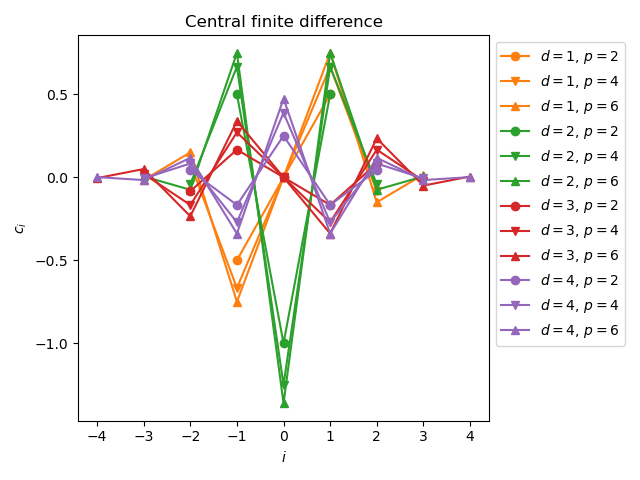
Make a plot of the coefficients depending on the indices.
maximum_differentiation_order = 4
formula_accuracy_list = [2, 4, 6]
direction = "central"
color_list = list(mcolors.TABLEAU_COLORS.keys())
marker_list = ["o", "v", "^", "<", ">"]
pl.figure()
pl.title("Central finite difference")
for differentiation_order in range(1, 1 + maximum_differentiation_order):
    for j in range(len(formula_accuracy_list)):
        finite_difference = nd.GeneralFiniteDifference(
            scaled_exp, x, differentiation_order, formula_accuracy_list[j], direction
        )
        coefficients = finite_difference.get_coefficients()
        imin, imax = finite_difference.get_indices_min_max()
        this_label = (
            r"$d = "
            f"{differentiation_order}"
            r"$, $p = "
            f"{formula_accuracy_list[j]}"
            r"$"
        )
        this_color = color_list[differentiation_order]
        this_marker = marker_list[j]
        pl.plot(
            range(imin, imax + 1),
            coefficients,
            "-" + this_marker,
            color=this_color,
            label=this_label,
        )
pl.xlabel(r"$i$")
pl.ylabel(r"$c_i$")
pl.legend(bbox_to_anchor=(1, 1))
pl.tight_layout()
Compute the coefficients of several forward F.D. formulas
We would like to compute the coefficients of a collection of forward finite difference formulas.
We consider the differentation order up to the sixth derivative and the forward F.D. formula up to the order 8.
maximum_differentiation_order = 6
formula_accuracy_list = list(range(1, 8))
We want to the print the result as a table. This is the reason why we need to align the coefficients on the columns on the table.
First pass: compute the maximum number of coefficients.
maximum_number_of_coefficients = 0
direction = "forward"
data = []
for differentiation_order in range(1, 1 + maximum_differentiation_order):
    for formula_accuracy in formula_accuracy_list:
        finite_difference = nd.GeneralFiniteDifference(
            scaled_exp, x, differentiation_order, formula_accuracy, direction
        )
        coefficients = finite_difference.get_coefficients()
        maximum_number_of_coefficients = max(
            maximum_number_of_coefficients, len(coefficients)
        )
        row = [differentiation_order, formula_accuracy]
        for i in range(len(coefficients)):
            row.append(f"{coefficients[i]:.3f}")
        data.append(row)
        index += 1
headers = ["Derivative", "Accuracy"]
for i in range(1 + maximum_number_of_coefficients):
    headers.append(i)
tabulate.tabulate(data, headers, tablefmt="html")
We notice that the sum of the coefficients is zero.
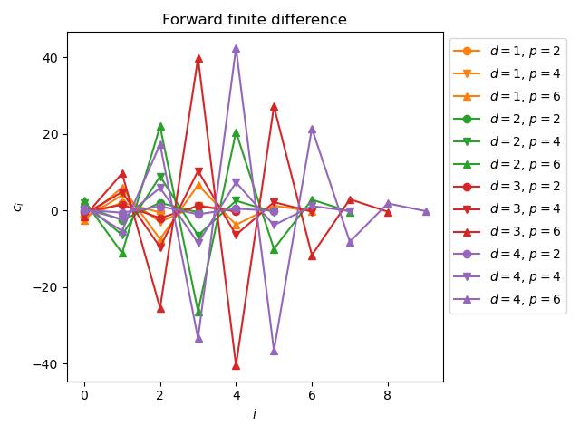
Make a plot of the coefficients depending on the indices.
maximum_differentiation_order = 4
formula_accuracy_list = [2, 4, 6]
direction = "forward"
color_list = list(mcolors.TABLEAU_COLORS.keys())
marker_list = ["o", "v", "^", "<", ">"]
pl.figure()
pl.title("Forward finite difference")
for differentiation_order in range(1, 1 + maximum_differentiation_order):
    for j in range(len(formula_accuracy_list)):
        finite_difference = nd.GeneralFiniteDifference(
            scaled_exp, x, differentiation_order, formula_accuracy_list[j], direction
        )
        coefficients = finite_difference.get_coefficients()
        imin, imax = finite_difference.get_indices_min_max()
        this_label = (
            r"$d = "
            f"{differentiation_order}"
            r"$, $p = "
            f"{formula_accuracy_list[j]}"
            r"$"
        )
        this_color = color_list[differentiation_order]
        this_marker = marker_list[j]
        pl.plot(
            range(imin, imax + 1),
            coefficients,
            "-" + this_marker,
            color=this_color,
            label=this_label,
        )
pl.xlabel(r"$i$")
pl.ylabel(r"$c_i$")
_ = pl.legend(bbox_to_anchor=(1, 1))
pl.tight_layout()
Total running time of the script: (0 minutes 0.400 seconds)