Convergence of the generalized finite differences formulas

This example shows the convergence properties of the generalized finite difference (F.D.) formulas.

The coefficients of the generalized finite difference formula are computed so that they approximate the derivative \(f^{(d)}(x)\) with order \(p\). More precisely, in exact arithmetic, we have:

\[f^{(d)}(x) = \frac{d!}{h^d} \sum_{i = i_{\min}}^{i_\max} c_i f(x + h i) + R(x; h)\]

where \(h > 0\) is the step, \(x\) is the point where the derivative is to be computed, \(d\) is the differentiation order and \(p\) is the order of accuracy of the formula, The remainder of the Taylor expansion is:

\[R(x; h) = - \frac{d!}{(d + p)!} b_{d + p} f^{(d + p)}(\xi) h^p.\]

where \(\xi \in (x, x + h)\) and the coefficient \(b_{d + p}\) is defined by the equation:

\[b_{d + p} = \sum_{i = i_{\min}}^{i_\max} i^{d + p} c_i.\]

The goal of this example is to show the actual behaviour of the remainder in floating point arithmetic for particular values of \(d\) and \(p\).

References

• 13. Baudin (2023). Méthodes numériques. Dunod.

import numpy as np
import numericalderivative as nd
import math
import pylab as pl

We consider the sinus function and we want to compute its first derivative i.e. \(d = 1\). We consider an order \(p = 2\) formula. Since \(d + p = 3\), the properties of the central finite difference formula depends on the third derivative of the function.

problem = nd.SinProblem()
name = problem.get_name()
first_derivative = problem.get_first_derivative()
third_derivative = problem.get_third_derivative()
function = problem.get_function()
x = problem.get_x()

We create the generalized central finite difference formula using GeneralFiniteDifference.

formula_accuracy = 2
differentiation_order = 1
formula = nd.GeneralFiniteDifference(
    function,
    x,
    differentiation_order,
    formula_accuracy,
    direction="central",
)

Compute the absolute error of approximate derivative i.e. \(\left|f^{(d)}(x) - \widetilde{f}^{(d)}(x)\right|\) where \(f^{(d)}(x)\) is the exact order \(d\) derivative of the function \(f\) and \(\widetilde{f}^{(d)}(x)\) is the approximation from the finite difference formula. Moreover, compute the absolute value of the remainder of the Taylor expansion, i.e. \(|R(x; h)|\). This requires to compute the constant \(b_{d + p}\), which is performed by compute_b_constant().

first_derivative_exact = first_derivative(x)
b_constant = formula.compute_b_constant()
scaled_b_parameter = (
    b_constant
    * math.factorial(differentiation_order)
    / math.factorial(differentiation_order + formula_accuracy)
)
number_of_steps = 50
step_array = np.logspace(-15, 1, number_of_steps)
abs_error_array = np.zeros((number_of_steps))
remainder_array = np.zeros((number_of_steps))
for i in range(number_of_steps):
    step = step_array[i]
    derivative_approx = formula.compute(step)
    abs_error_array[i] = abs(derivative_approx - first_derivative_exact)
    remainder_array[i] = (
        abs(scaled_b_parameter * third_derivative(x)) * step**formula_accuracy
    )

pl.figure()
pl.title(
    f"Derivative of {name} at x={x}, "
    f"d={differentiation_order}, p={formula_accuracy}"
)
pl.plot(step_array, abs_error_array, "o--", label="Abs. error")
pl.plot(step_array, remainder_array, "^:", label="Abs. remainder")
pl.xlabel("Step h")
pl.ylabel("Absolute error")
pl.xscale("log")
pl.yscale("log")
_ = pl.legend()

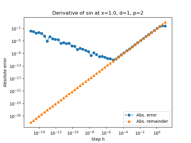
We see that there is a good agreement between the model and the actual error when the step size is sufficiently large. When the step is close to zero however, the rounding errors increase the absolute error and the model does not fit anymore.