Note
Go to the end to download the full example code.
Experiments with Dumontet & Vignes method
References
Dumontet, J., & Vignes, J. (1977). Détermination du pas optimal dans le calcul des dérivées sur ordinateur. RAIRO. Analyse numérique, 11 (1), 13-25.
import numpy as np
import pylab as pl
import numericalderivative as nd
import sys
from matplotlib.ticker import MaxNLocator
Use the method on a simple problem
In the next example, we use the algorithm on the exponential function.
We create the DumontetVignes algorithm using the function and the point x.
Then we use the find_step() method to compute the step,
using an upper bound of the step as an initial point of the algorithm.
Finally, use the compute_first_derivative() method to compute
an approximate value of the first derivative using finite differences.
The get_number_of_function_evaluations() method
can be used to get the number of function evaluations.
x = 1.0
kmin = 1.0e-10
kmax = 1.0e0
algorithm = nd.DumontetVignes(np.exp, x, verbose=True)
step, number_of_iterations = algorithm.find_step(kmin=kmin, kmax=kmax)
f_prime_approx = algorithm.compute_first_derivative(step)
feval = algorithm.get_number_of_function_evaluations()
f_prime_exact = np.exp(x)  # Since the derivative of exp is exp.
print(f"Computed step = {step:.3e}")
print(f"Number of iterations = {number_of_iterations}")
print(f"f_prime_approx = {f_prime_approx}")
print(f"f_prime_exact = {f_prime_exact}")
absolute_error = abs(f_prime_approx - f_prime_exact)
x = 1.000e+00
iteration_maximum = 53
kmin =  1e-10
kmax =  1.0
L(kmin) =  -1.0
L(kmax) =  1.0000000000000113
+ Iteration = 0, kmin = 1.000e-10, kmax = 1.000e+00
  k = 5.000e-01, f3inf = 2.892e+00, f3sup = 2.892e+00, ell = 1.000e+00
  k is too large : reduce kmax
+ Iteration = 1, kmin = 1.000e-10, kmax = 5.000e-01
  k = 2.500e-01, f3inf = 2.761e+00, f3sup = 2.761e+00, ell = 1.000e+00
  k is too large : reduce kmax
+ Iteration = 2, kmin = 1.000e-10, kmax = 2.500e-01
  k = 1.250e-01, f3inf = 2.729e+00, f3sup = 2.729e+00, ell = 1.000e+00
  k is too large : reduce kmax
+ Iteration = 3, kmin = 1.000e-10, kmax = 1.250e-01
  k = 6.250e-02, f3inf = 2.721e+00, f3sup = 2.721e+00, ell = 1.000e+00
  k is too large : reduce kmax
+ Iteration = 4, kmin = 1.000e-10, kmax = 6.250e-02
  k = 3.125e-02, f3inf = 2.719e+00, f3sup = 2.719e+00, ell = 1.000e+00
  k is too large : reduce kmax
+ Iteration = 5, kmin = 1.000e-10, kmax = 3.125e-02
  k = 1.563e-02, f3inf = 2.718e+00, f3sup = 2.718e+00, ell = 1.000e+00
  k is too large : reduce kmax
+ Iteration = 6, kmin = 1.000e-10, kmax = 1.563e-02
  k = 7.813e-03, f3inf = 2.718e+00, f3sup = 2.718e+00, ell = 1.000e+00
  k is too large : reduce kmax
+ Iteration = 7, kmin = 1.000e-10, kmax = 7.813e-03
  k = 3.906e-03, f3inf = 2.718e+00, f3sup = 2.718e+00, ell = 1.000e+00
  k is too large : reduce kmax
+ Iteration = 8, kmin = 1.000e-10, kmax = 3.906e-03
  k = 1.953e-03, f3inf = 2.718e+00, f3sup = 2.718e+00, ell = 1.000e+00
  k is too large : reduce kmax
+ Iteration = 9, kmin = 1.000e-10, kmax = 1.953e-03
  k = 9.766e-04, f3inf = 2.718e+00, f3sup = 2.718e+00, ell = 1.000e+00
  k is too large : reduce kmax
+ Iteration = 10, kmin = 1.000e-10, kmax = 9.766e-04
  k = 4.883e-04, f3inf = 2.718e+00, f3sup = 2.718e+00, ell = 1.000e+00
  k is too large : reduce kmax
+ Iteration = 11, kmin = 1.000e-10, kmax = 4.883e-04
  k = 2.441e-04, f3inf = 2.718e+00, f3sup = 2.719e+00, ell = 1.000e+00
  k is too large : reduce kmax
+ Iteration = 12, kmin = 1.000e-10, kmax = 2.441e-04
  k = 1.221e-04, f3inf = 2.713e+00, f3sup = 2.723e+00, ell = 1.004e+00
  k is too large : reduce kmax
+ Iteration = 13, kmin = 1.000e-10, kmax = 1.221e-04
  k = 6.104e-05, f3inf = 2.680e+00, f3sup = 2.758e+00, ell = 1.029e+00
  k is too large : reduce kmax
+ Iteration = 14, kmin = 1.000e-10, kmax = 6.104e-05
  k = 3.052e-05, f3inf = 2.406e+00, f3sup = 3.031e+00, ell = 1.260e+00
  k is too large : reduce kmax
+ Iteration = 15, kmin = 1.000e-10, kmax = 3.052e-05
Warning: f3inf is zero!
  k = 1.526e-05, f3inf = 0.000e+00, f3sup = 5.000e+00, ell = inf
  k is too small : increase kmin
+ Iteration = 16, kmin = 1.526e-05, kmax = 3.052e-05
  k = 2.289e-05, f3inf = 1.926e+00, f3sup = 3.407e+00, ell = 1.769e+00
  k is too large : reduce kmax
+ Iteration = 17, kmin = 1.526e-05, kmax = 2.289e-05
  k = 1.907e-05, f3inf = 1.536e+00, f3sup = 4.096e+00, ell = 2.667e+00
  k is OK : stop
Computed step = 1.021e-05
Number of iterations = 17
f_prime_approx = 2.7182818285157593
f_prime_exact = 2.718281828459045
Useful functions
These functions will be used later in this example.
def compute_ell(function, x, k, relative_precision):
    """
    Compute the L ratio for a given value of the step k.
    """
    algorithm = nd.DumontetVignes(function, x, relative_precision=relative_precision)
    ell = algorithm.compute_ell(k)
    return ell


def compute_f3_inf_sup(function, x, k, relative_precision):
    """
    Compute the upper and lower bounds of the third derivative for a given value of k.
    """
    algorithm = nd.DumontetVignes(function, x, relative_precision=relative_precision)
    _, f3inf, f3sup = algorithm.compute_ell(k)
    return f3inf, f3sup


def plot_step_sensitivity(
    x,
    name,
    function,
    function_derivative,
    function_third_derivative,
    step_array,
    iteration_maximum=53,
    relative_precision=1.0e-15,
    kmin=None,
    kmax=None,
):
    """
    Create a plot representing the absolute error depending on step.

    Compute the approximate derivative using central F.D. formula.
    Plot the approximately optimal step computed by DumontetVignes.

    Parameters
    ----------
    x : float
        The input point
    name : str
        The name of the problem
    function : function
        The function.
    function_derivative : function
        The exact first derivative of the function.
    function_third_derivative : function
        The exact third derivative of the function.
    step_array : array(n_points)
        The array of steps to consider
    iteration_maximum : int
        The maximum number of iterations in DumontetVignes
    relative_precision : float, > 0
        The relative precision of the function evaluation
    kmin : float, kmin > 0
        A minimum bound for k. The default is None.
        If no value is provided, the default is to compute the smallest
        possible kmin using number_of_digits and x.
    kmax : float, kmax > kmin > 0
        A maximum bound for k. The default is None.
        If no value is provided, the default is to compute the largest
        possible kmax using number_of_digits and x.
    """
    print("+ ", name)
    # 1. Plot the error vs h
    algorithm = nd.DumontetVignes(function, x, verbose=True)
    number_of_points = len(step_array)
    error_array = np.zeros((number_of_points))
    for i in range(number_of_points):
        f_prime_approx = algorithm.compute_first_derivative(step_array[i])
        error_array[i] = abs(f_prime_approx - function_derivative(x))

    # 2. Algorithm to detect h*
    algorithm = nd.DumontetVignes(function, x, relative_precision=relative_precision)
    print("Exact f'''(x) = %.3e" % (function_third_derivative(x)))
    estim_step, _ = algorithm.find_step(
        iteration_maximum=iteration_maximum,
        kmin=kmin,
        kmax=kmax,
    )
    fprime = algorithm.compute_first_derivative(estim_step)
    number_of_function_evaluations = algorithm.get_number_of_function_evaluations()
    print("Function evaluations =", number_of_function_evaluations)
    print("Estim. derivative = %.3e" % (fprime))
    print("Exact. derivative = %.3e" % (function_derivative(x)))
    f_prime_approx = algorithm.compute_first_derivative(estim_step)
    absolute_error = abs(f_prime_approx - function_derivative(x))
    print("Exact abs. error  = %.3e" % (absolute_error))
    print("Exact rel. error  = %.3e" % (absolute_error / abs(function_derivative(x))))
    # Compute exact step
    absolute_precision = abs(function(x) * relative_precision)
    third_derivative_value = function_third_derivative(x)
    optimal_step, optimal_error = nd.FirstDerivativeCentral.compute_step(
        third_derivative_value, absolute_precision
    )
    print("Exact step     = %.3e" % (optimal_step))
    print("Estimated step = %.3e" % (estim_step))
    print("Optimal abs. error = %.3e" % (optimal_error))
    print("Optimal rel. error = %.3e" % (optimal_error / abs(function_derivative(x))))

    minimum_error = np.nanmin(error_array)
    maximum_error = np.nanmax(error_array)

    pl.figure()
    pl.plot(step_array, error_array)
    pl.plot(
        [estim_step] * 2, [minimum_error, maximum_error], "--", label=r"$\widetilde{h}$"
    )
    pl.plot(optimal_step, optimal_error, "o", label=r"$h^\star$")
    pl.title("Finite difference for %s" % (name))
    pl.xlabel("h")
    pl.ylabel("Error")
    pl.xscale("log")
    pl.yscale("log")
    pl.legend(bbox_to_anchor=(1.1, 1.0))
    pl.tight_layout()
    return
def plot_ell_ratio(
    name,
    function,
    x,
    number_of_points,
    number_of_digits,
    relative_precision,
    kmin=None,
    kmax=None,
    y_logscale=False,
    plot_L_constants=True,
    epsilon_ell=1.0e-5,
):
    """Plot the ell ratio depending on the step size.

    This ell ratio is used in DumontetVignes."""
    ell_1 = 1.0 / 15.0  # Eq. 34, fixed
    ell_2 = 1.0 / 2.0
    ell_3 = 1.0 / ell_2
    ell_4 = 1.0 / ell_1

    if kmin is None:
        print("Set default kmin")
        kmin = x * 2 ** (-number_of_digits + 1)  # Eq. 26
    if kmax is None:
        print("Set default kmax")
        kmax = x * 2 ** (number_of_digits - 1)
    k_array = np.logspace(np.log10(kmin), np.log10(kmax), number_of_points)
    ell_array = np.zeros((number_of_points))
    for i in range(number_of_points):
        ell_array[i], _, _ = compute_ell(function, x, k_array[i], relative_precision)

    fig = pl.figure()
    pl.plot(k_array, ell_array, label="L")
    if plot_L_constants:
        indices = np.isfinite(ell_array)
        maximum_finite_ell = np.max(ell_array[indices])
        print(
            f"maximum_finite_ell = {maximum_finite_ell}, "
            f"maximum_finite_ell - 1 = {maximum_finite_ell - 1}"
        )

        if maximum_finite_ell <= 1.0 + epsilon_ell:
            print("maximum L is lower or equal to 1")
            pl.plot(
                k_array, [ell_1] * number_of_points, "--", label=f"$L_1$ = {ell_1:.3f}"
            )
            pl.plot(
                k_array, [ell_2] * number_of_points, ":", label=f"$L_2$ = {ell_2:.3f}"
            )
        else:
            print("maximum L is greater than 1")
            pl.plot(
                k_array, [ell_3] * number_of_points, ":", label=f"$L_3$ = {ell_3:.3f}"
            )
            pl.plot(
                k_array, [ell_4] * number_of_points, "--", label=f"$L_4$ = {ell_4:.3f}"
            )
        pl.legend(bbox_to_anchor=(1.0, 1.0))
    pl.title(f"{name}, x = {x:.2e}, p = {relative_precision:.2e}")
    pl.xlabel("k")
    pl.ylabel("L")
    pl.xscale("log")
    if y_logscale:
        pl.yscale("log")
    #
    pl.tight_layout()
    return
Plot the L ratio for various problems
The L ratio is the criterion used in (Dumontet & Vignes, 1977) algorithm
to find a satisfactory step k.
The algorithm searches for a step k so that the L ratio is inside
an interval.
This is computed by the compute_ell()
method.
In the next examples, we plot the L ratio depending on k
for different functions.
Consider the
ExponentialProblemfunction.
problem = nd.ExponentialProblem()
x = problem.get_x()
problem
number_of_points = 200
relative_precision = 1.0e-15
number_of_digits = 53
plot_ell_ratio(
    problem.get_name(),
    problem.get_function(),
    x,
    number_of_points,
    number_of_digits,
    relative_precision,
    kmin=1.0e-7,
    kmax=1.0e-3,
    plot_L_constants=True,
)
_ = pl.ylim(-20.0, 20.0)
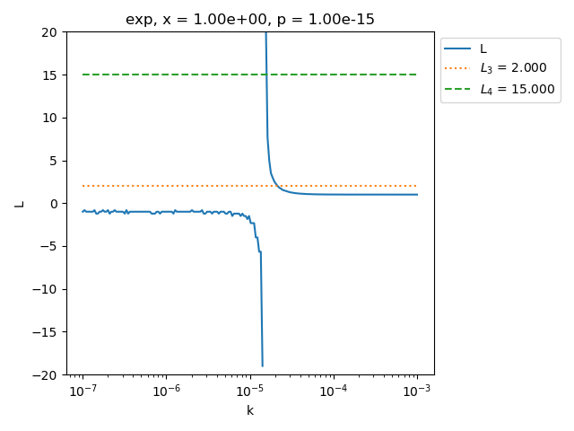
maximum_finite_ell = 20.999999999999996, maximum_finite_ell - 1 = 19.999999999999996
maximum L is greater than 1
See how the figure changes when the relative precision is increased: use 1.e-14 (instead of 1.e-15 in the previous example).
relative_precision = 1.0e-14
number_of_digits = 53
plot_ell_ratio(
    problem.get_name(),
    problem.get_function(),
    x,
    number_of_points,
    number_of_digits,
    relative_precision,
    kmin=1.0e-7,
    kmax=1.0e-3,
    plot_L_constants=True,
)
_ = pl.ylim(-20.0, 20.0)
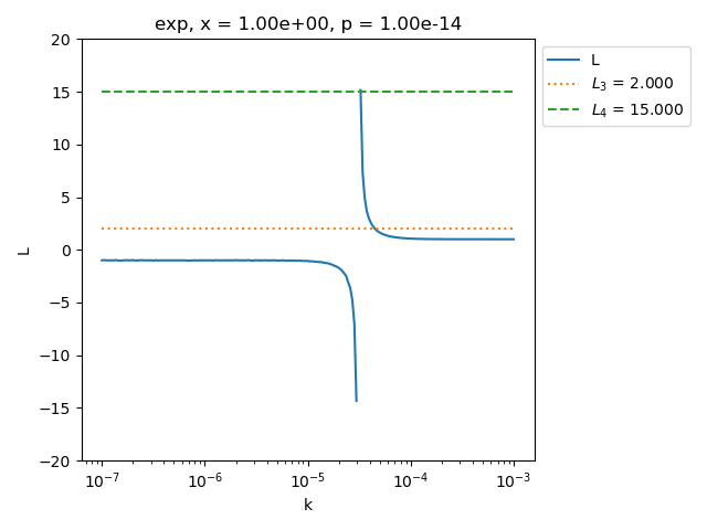
maximum_finite_ell = 15.153846153846153, maximum_finite_ell - 1 = 14.153846153846153
maximum L is greater than 1
See what happens when the relative precision is reduced: here 1.e-16 instead of 1.e-14 in the previous example.
relative_precision = 1.0e-16
number_of_digits = 53
plot_ell_ratio(
    problem.get_name(),
    problem.get_function(),
    x,
    number_of_points,
    number_of_digits,
    relative_precision,
    kmin=1.0e-7,
    kmax=1.0e-3,
)
_ = pl.ylim(-20.0, 20.0)
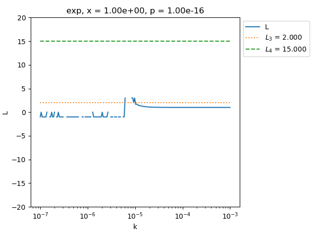
maximum_finite_ell = 3.0, maximum_finite_ell - 1 = 2.0
maximum L is greater than 1
We see that it is difficult to find a value of k such that L(k) is in the required interval when the relative precision is too close to zero.
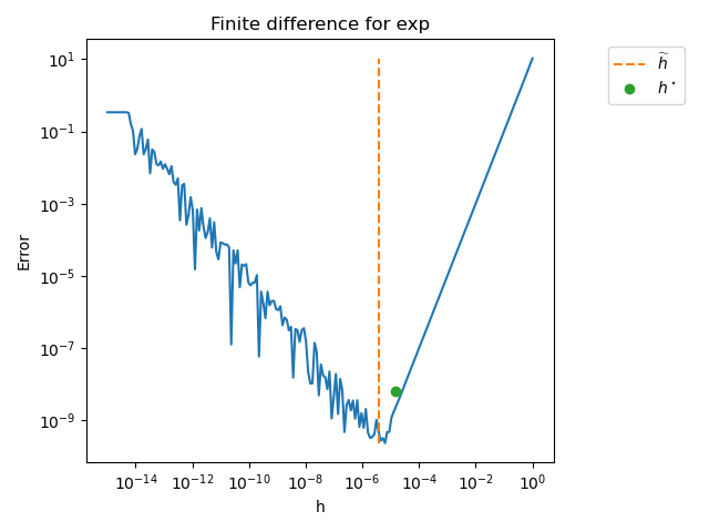
Plot the error depending on the step
In the next examples, we plot the error of the approximation of the first derivative by the finite difference formula depending on the step size.
x = 4.0
problem = nd.ExponentialProblem()
function = problem.get_function()
absolute_precision = sys.float_info.epsilon * function(x)
print("absolute_precision = %.3e" % (absolute_precision))
absolute_precision = 1.212e-14
x = 4.1  # A carefully chosen point
relative_precision = sys.float_info.epsilon
number_of_points = 200
step_array = np.logspace(-15.0, 0.0, number_of_points)
kmin = 1.0e-5
kmax = 1.0e-2
plot_step_sensitivity(
    x,
    problem.get_name(),
    problem.get_function(),
    problem.get_first_derivative(),
    problem.get_third_derivative(),
    step_array,
    iteration_maximum=20,
    relative_precision=1.0e-15,
    kmin=kmin,
    kmax=kmax,
)
+  exp
Exact f'''(x) = 6.034e+01
Function evaluations = 50
Estim. derivative = 6.034e+01
Exact. derivative = 6.034e+01
Exact abs. error  = 2.184e-10
Exact rel. error  = 3.619e-12
Exact step     = 1.442e-05
Estimated step = 3.705e-06
Optimal abs. error = 6.276e-09
Optimal rel. error = 1.040e-10
In the previous figure, we see that the error reaches
a minimum, which is indicated by the green point labeled \(h^\star\).
The vertical dotted line represents the approximately optimal step \(\widetilde{h}\)
returned by the find_step() method.
We see that the method correctly computes an approximation of the the optimal step.
Consider the ScaledExponentialProblem.
First, we plot the L ratio.
relative_precision = 1.0e-14
problem = nd.ScaledExponentialProblem()
number_of_digits = 53
plot_ell_ratio(
    problem.get_name(),
    problem.get_function(),
    problem.get_x(),
    number_of_points,
    number_of_digits,
    relative_precision,
    kmin=1.0e-1,
    kmax=1.0e2,
    plot_L_constants=True,
)
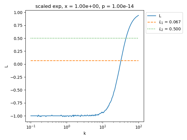
maximum_finite_ell = 0.9422164726175075, maximum_finite_ell - 1 = -0.05778352738249248
maximum L is lower or equal to 1
Then plot the error depending on the step size.
problem = nd.ScaledExponentialProblem()
step_array = np.logspace(-7.0, 6.0, number_of_points)
plot_step_sensitivity(
    problem.get_x(),
    problem.get_name(),
    problem.get_function(),
    problem.get_first_derivative(),
    problem.get_third_derivative(),
    step_array,
    relative_precision=1.0e-15,
    kmin=1.0e-2,
    kmax=1.0e2,
)
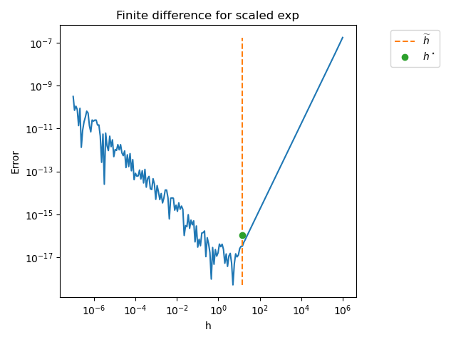
+  scaled exp
Exact f'''(x) = -1.000e-18
Function evaluations = 26
Estim. derivative = -1.000e-06
Exact. derivative = -1.000e-06
Exact abs. error  = 3.405e-17
Exact rel. error  = 3.405e-11
Exact step     = 1.442e+01
Estimated step = 1.438e+01
Optimal abs. error = 1.040e-16
Optimal rel. error = 1.040e-10
The previous figure shows that the optimal step is close to \(10^1\), which may be larger than what we may typically expect as a step size for a finite difference formula.
Compute the lower and upper bounds of the third derivative
The algorithm is based on bounds of the third derivative, which is
computed by the compute_ell() method.
These bounds are used to find a step which is approximately
optimal to compute the step of the finite difference formula
used for the first derivative.
Hence, it is interesting to compare the bounds computed
by the (Dumontet & Vignes, 1977) algorithm and the
actual value of the third derivative.
To compute the true value of the third derivative,
we use two different methods:
a finite difference formula, using
ThirdDerivativeCentral,the exact third derivative, using
get_third_derivative().
x = 1.0
k = 1.0e-3  # A first guess
print("x = ", x)
print("k = ", k)
problem = nd.SquareRootProblem()
function = problem.get_function()
finite_difference = nd.ThirdDerivativeCentral(function, x)
approx_f3d = finite_difference.compute(k)
print("Approx. f''(x) = ", approx_f3d)
third_derivative = problem.get_third_derivative()
exact_f3d = third_derivative(x)
print("Exact f''(x) = ", exact_f3d)
x =  1.0
k =  0.001
Approx. f''(x) =  0.37500080818375636
Exact f''(x) =  0.375
relative_precision = 1.0e-14
print("relative_precision = ", relative_precision)
function = problem.get_function()
f3inf, f3sup = compute_f3_inf_sup(function, x, k, relative_precision)
print("f3inf = ", f3inf)
print("f3sup = ", f3sup)
relative_precision =  1e-14
f3inf =  0.37497116522899887
f3sup =  0.3750306731831188
The previous outputs shows that the lower and upper bounds computed by the algorithm contain, indeed, the true value of the third derivative in this case.
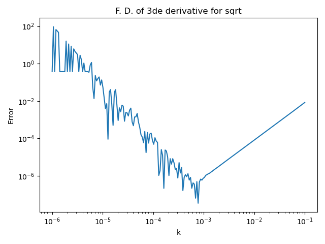
The algorithm is based on finding an approximatly optimal step k to compute the third derivative. The next script computes the error of the central formula for the finite difference formula depending on the step k.
number_of_points = 200
function = problem.get_function()
third_derivative = problem.get_third_derivative()
k_array = np.logspace(-6.0, -1.0, number_of_points)
error_array = np.zeros((number_of_points))
algorithm = nd.ThirdDerivativeCentral(function, x)
for i in range(number_of_points):
    f2nde_approx = algorithm.compute(k_array[i])
    error_array[i] = abs(f2nde_approx - third_derivative(x))
pl.figure()
pl.plot(k_array, error_array)
pl.title("F. D. of 3de derivative for %s" % (problem.get_name()))
pl.xlabel("k")
pl.ylabel("Error")
pl.xscale("log")
pl.yscale("log")
#
pl.tight_layout()
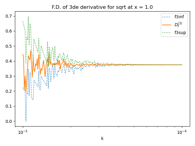
Plot the lower and upper bounds of the third derivative
The next figure presents the sensitivity of the lower and upper bounds of the third derivative to the step k. Moreover, it presents the approximation of the third derivative using the central finite difference formula. This makes it possible to check that the lower and upper bounds actually contain the approximation produced by the F.D. formula.
problem = nd.SquareRootProblem()
number_of_points = 200
relative_precision = 1.0e-16
k_array = np.logspace(-5.0, -4.0, number_of_points)
f3_array = np.zeros((number_of_points, 3))
function = problem.get_function()
algorithm = nd.ThirdDerivativeCentral(function, x)
for i in range(number_of_points):
    f3inf, f3sup = compute_f3_inf_sup(function, x, k_array[i], relative_precision)
    f3_approx = algorithm.compute(k_array[i])
    f3_array[i] = [f3inf, f3_approx, f3sup]
pl.figure()
pl.plot(k_array, f3_array[:, 0], ":", label="f3inf")
pl.plot(k_array, f3_array[:, 1], "-", label="$D^{(3)}_f$")
pl.plot(k_array, f3_array[:, 2], ":", label="f3sup")
pl.title(f"F.D. of 3de derivative for {problem.get_name()} at x = {x}")
pl.xlabel("k")
pl.xscale("log")
pl.legend(bbox_to_anchor=(1.0, 1.0))
pl.tight_layout(pad=1.2)
x = 1.0e-2
relative_precision = 1.0e-14
number_of_digits = 53
plot_ell_ratio(
    problem.get_name(),
    problem.get_function(),
    x,
    number_of_points,
    number_of_digits,
    relative_precision,
    kmin=4.4e-7,
    kmax=1.0e-5,
    plot_L_constants=True,
)
_ = pl.ylim(-20.0, 20.0)
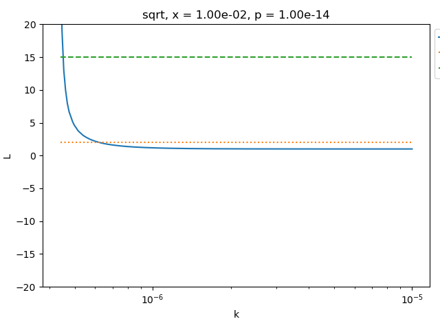
maximum_finite_ell = 31.85714285714286, maximum_finite_ell - 1 = 30.85714285714286
maximum L is greater than 1
The next example searches the optimal step for the square root function.
x = 1.0e-2
relative_precision = 1.0e-14
kmin = 1.0e-8
kmax = 1.0e-3
verbose = True
function = problem.get_function()
algorithm = nd.DumontetVignes(
    function, x, relative_precision=relative_precision, verbose=verbose
)
h_optimal, _ = algorithm.find_step(kmax=kmax)
print("h optimal = %.3e" % (h_optimal))
number_of_feval = algorithm.get_number_of_function_evaluations()
print(f"number_of_feval = {number_of_feval}")
f_prime_approx = algorithm.compute_first_derivative(h_optimal)
feval = algorithm.get_number_of_function_evaluations()
first_derivative = problem.get_first_derivative()
absolute_error = abs(f_prime_approx - first_derivative(x))
print("Abs. error = %.3e" % (absolute_error))

ell_kmin, f3inf, f3sup = algorithm.compute_ell(kmin)
print("L(kmin) = ", ell_kmin)
ell_kmax, f3inf, f3sup = algorithm.compute_ell(kmax)
print("L(kmax) = ", ell_kmax)
x = 1.000e-02
iteration_maximum = 53
kmin =  2.220446049250313e-18
kmax =  0.001
L(kmin) =  -1.0186915887850467
L(kmax) =  1.0000000001563647
+ Iteration = 0, kmin = 2.220e-18, kmax = 1.000e-03
  k = 5.000e-04, f3inf = 3.771e+04, f3sup = 3.771e+04, ell = 1.000e+00
  k is too large : reduce kmax
+ Iteration = 1, kmin = 2.220e-18, kmax = 5.000e-04
  k = 2.500e-04, f3inf = 3.755e+04, f3sup = 3.755e+04, ell = 1.000e+00
  k is too large : reduce kmax
+ Iteration = 2, kmin = 2.220e-18, kmax = 2.500e-04
  k = 1.250e-04, f3inf = 3.751e+04, f3sup = 3.751e+04, ell = 1.000e+00
  k is too large : reduce kmax
+ Iteration = 3, kmin = 2.220e-18, kmax = 1.250e-04
  k = 6.250e-05, f3inf = 3.750e+04, f3sup = 3.750e+04, ell = 1.000e+00
  k is too large : reduce kmax
+ Iteration = 4, kmin = 2.220e-18, kmax = 6.250e-05
  k = 3.125e-05, f3inf = 3.750e+04, f3sup = 3.750e+04, ell = 1.000e+00
  k is too large : reduce kmax
+ Iteration = 5, kmin = 2.220e-18, kmax = 3.125e-05
  k = 1.563e-05, f3inf = 3.750e+04, f3sup = 3.750e+04, ell = 1.000e+00
  k is too large : reduce kmax
+ Iteration = 6, kmin = 2.220e-18, kmax = 1.563e-05
  k = 7.813e-06, f3inf = 3.749e+04, f3sup = 3.751e+04, ell = 1.000e+00
  k is too large : reduce kmax
+ Iteration = 7, kmin = 2.220e-18, kmax = 7.813e-06
  k = 3.906e-06, f3inf = 3.745e+04, f3sup = 3.755e+04, ell = 1.003e+00
  k is too large : reduce kmax
+ Iteration = 8, kmin = 2.220e-18, kmax = 3.906e-06
  k = 1.953e-06, f3inf = 3.710e+04, f3sup = 3.790e+04, ell = 1.022e+00
  k is too large : reduce kmax
+ Iteration = 9, kmin = 2.220e-18, kmax = 1.953e-06
  k = 9.766e-07, f3inf = 3.427e+04, f3sup = 4.071e+04, ell = 1.188e+00
  k is too large : reduce kmax
+ Iteration = 10, kmin = 2.220e-18, kmax = 9.766e-07
  k = 4.883e-07, f3inf = 1.168e+04, f3sup = 6.318e+04, ell = 5.408e+00
  k is OK : stop
h optimal = 4.311e-07
number_of_feval = 52
Abs. error = 1.151e-09
L(kmin) =  -1.0
L(kmax) =  1.0000000001563647
Consider the SinProblem.
x = 1.0
relative_precision = 1.0e-14
problem = nd.SinProblem()
function = problem.get_function()
name = "sin"
number_of_digits = 53
kmin = 1.0e-5
kmax = 1.0e-3
plot_ell_ratio(
    name,
    function,
    x,
    number_of_points,
    number_of_digits,
    relative_precision,
    kmin=kmin,
    kmax=kmax,
    plot_L_constants=True,
)
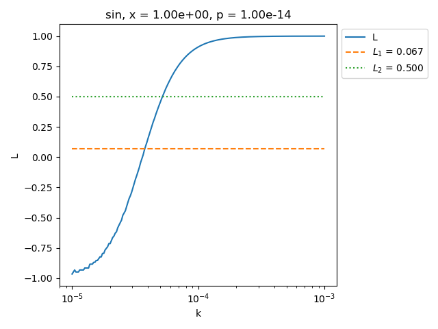
maximum_finite_ell = 0.9999063046299485, maximum_finite_ell - 1 = -9.369537005154971e-05
maximum L is lower or equal to 1
x = 1.0
k = 1.0e-3
print("x = ", x)
print("k = ", k)
function = problem.get_function()
algorithm = nd.ThirdDerivativeCentral(function, x)
approx_f3d = algorithm.compute(k)
print("Approx. f''(x) = ", approx_f3d)
third_derivative = problem.get_third_derivative()
exact_f3d = third_derivative(x)
print("Exact f''(x) = ", exact_f3d)
relative_precision = 1.0e-14
print("relative_precision = ", relative_precision)
function = problem.get_function()
f3inf, f3sup = compute_f3_inf_sup(function, x, k, relative_precision)
print("f3inf = ", f3inf)
print("f3sup = ", f3sup)
x =  1.0
k =  0.001
Approx. f''(x) =  -0.5403020253424984
Exact f''(x) =  -0.5403023058681398
relative_precision =  1e-14
f3inf =  -0.5403273384274598
f3sup =  -0.5402767122575369
See the history of steps during the bissection search
In Dumontet & Vignes's method, the bisection algorithm
produces a sequence of steps \((k_i)_{1 \leq i \leq n_{iter}}\)
where \(n_{iter} \in \mathbb{N}\) is the number of iterations.
These steps are meant to converge to an
approximately optimal step of for the central finite difference formula of the
third derivative.
The optimal step \(k^\star\) for the central finite difference formula of the
third derivative can be computed depending on the fifth derivative of the
function.
In the next example, we want to compute the absolute error between
each intermediate step \(k_i\) and the exact value \(k^\star\)
to see how close the algorithm gets to the exact step.
The list of intermediate steps during the algorithm can be obtained
thanks to the get_step_history() method.
In the next example, we print the intermediate steps k during the bissection algorithm that searches for a step such that the L ratio is satisfactory.
problem = nd.SinProblem()
function = problem.get_function()
name = problem.get_name()
x = problem.get_x()
algorithm = nd.DumontetVignes(function, x, verbose=True)
kmin = 1.0e-10
kmax = 1.0e0
step, number_of_iterations = algorithm.find_step(kmin=kmin, kmax=kmax)
step_k_history = algorithm.get_step_history()
print(f"Number of iterations = {number_of_iterations}")
print(f"History of steps k : {step_k_history}")
last_step_k = step_k_history[-1]
print(f"Last step k : {last_step_k}")
x = 1.000e+00
iteration_maximum = 53
kmin =  1e-10
kmax =  1.0
L(kmin) =  -1.0
L(kmax) =  0.999999999999993
+ Iteration = 0, kmin = 1.000e-10, kmax = 1.000e+00
  k = 5.000e-01, f3inf = -5.074e-01, f3sup = -5.074e-01, ell = 1.000e+00
  k is too large : reduce kmax
+ Iteration = 1, kmin = 1.000e-10, kmax = 5.000e-01
  k = 2.500e-01, f3inf = -5.319e-01, f3sup = -5.319e-01, ell = 1.000e+00
  k is too large : reduce kmax
+ Iteration = 2, kmin = 1.000e-10, kmax = 2.500e-01
  k = 1.250e-01, f3inf = -5.382e-01, f3sup = -5.382e-01, ell = 1.000e+00
  k is too large : reduce kmax
+ Iteration = 3, kmin = 1.000e-10, kmax = 1.250e-01
  k = 6.250e-02, f3inf = -5.398e-01, f3sup = -5.398e-01, ell = 1.000e+00
  k is too large : reduce kmax
+ Iteration = 4, kmin = 1.000e-10, kmax = 6.250e-02
  k = 3.125e-02, f3inf = -5.402e-01, f3sup = -5.402e-01, ell = 1.000e+00
  k is too large : reduce kmax
+ Iteration = 5, kmin = 1.000e-10, kmax = 3.125e-02
  k = 1.563e-02, f3inf = -5.403e-01, f3sup = -5.403e-01, ell = 1.000e+00
  k is too large : reduce kmax
+ Iteration = 6, kmin = 1.000e-10, kmax = 1.563e-02
  k = 7.813e-03, f3inf = -5.403e-01, f3sup = -5.403e-01, ell = 1.000e+00
  k is too large : reduce kmax
+ Iteration = 7, kmin = 1.000e-10, kmax = 7.813e-03
  k = 3.906e-03, f3inf = -5.403e-01, f3sup = -5.403e-01, ell = 1.000e+00
  k is too large : reduce kmax
+ Iteration = 8, kmin = 1.000e-10, kmax = 3.906e-03
  k = 1.953e-03, f3inf = -5.403e-01, f3sup = -5.403e-01, ell = 1.000e+00
  k is too large : reduce kmax
+ Iteration = 9, kmin = 1.000e-10, kmax = 1.953e-03
  k = 9.766e-04, f3inf = -5.403e-01, f3sup = -5.403e-01, ell = 1.000e+00
  k is too large : reduce kmax
+ Iteration = 10, kmin = 1.000e-10, kmax = 9.766e-04
  k = 4.883e-04, f3inf = -5.403e-01, f3sup = -5.403e-01, ell = 9.999e-01
  k is too large : reduce kmax
+ Iteration = 11, kmin = 1.000e-10, kmax = 4.883e-04
  k = 2.441e-04, f3inf = -5.405e-01, f3sup = -5.401e-01, ell = 9.993e-01
  k is too large : reduce kmax
+ Iteration = 12, kmin = 1.000e-10, kmax = 2.441e-04
  k = 1.221e-04, f3inf = -5.417e-01, f3sup = -5.388e-01, ell = 9.946e-01
  k is too large : reduce kmax
+ Iteration = 13, kmin = 1.000e-10, kmax = 1.221e-04
  k = 6.104e-05, f3inf = -5.518e-01, f3sup = -5.283e-01, ell = 9.575e-01
  k is too large : reduce kmax
+ Iteration = 14, kmin = 1.000e-10, kmax = 6.104e-05
  k = 3.052e-05, f3inf = -6.328e-01, f3sup = -4.453e-01, ell = 7.037e-01
  k is too large : reduce kmax
+ Iteration = 15, kmin = 1.000e-10, kmax = 3.052e-05
  k = 1.526e-05, f3inf = -1.312e+00, f3sup = 1.875e-01, ell = -1.429e-01
  k is too small : increase kmin
+ Iteration = 16, kmin = 1.526e-05, kmax = 3.052e-05
  k = 2.289e-05, f3inf = -7.778e-01, f3sup = -3.333e-01, ell = 4.286e-01
  k is OK : stop
Number of iterations = 16
History of steps k : [0.50000000005, 0.250000000075, 0.1250000000875, 0.06250000009375001, 0.031250000096875, 0.0156250000984375, 0.007812500099218751, 0.0039062500996093754, 0.0019531250998046875, 0.0009765625999023438, 0.0004882813499511719, 0.00024414072497558597, 0.00012207041248779297, 6.103525624389649e-05, 3.051767812194824e-05, 1.525888906097412e-05, 2.288828359146118e-05]
Last step k : 2.288828359146118e-05
Then we compute the exact step, using compute_step().
fifth_derivative = problem.get_fifth_derivative()
fifth_derivative_value = fifth_derivative(x)
print(f"f^(5)(x) = {fifth_derivative_value}")
absolute_precision = 1.0e-16
exact_step_k, absolute_error = nd.ThirdDerivativeCentral.compute_step(
    fifth_derivative_value, absolute_precision
)
print(f"Optimal step k for f^(3)(x) = {exact_step_k}")
f^(5)(x) = 0.5403023058681398
Optimal step k for f^(3)(x) = 0.0012721172356439541
Plot the absolute error between the exact step k and the intermediate k of the algorithm.
error_step_k = [
    abs(step_k_history[i] - exact_step_k) for i in range(len(step_k_history))
]
fig = pl.figure()
pl.title(f"Dumontet & Vignes on {name} at x = {x}")
pl.plot(range(len(step_k_history)), error_step_k, "o-")
pl.xlabel("Iterations")
pl.ylabel(r"$|k_i - k^\star|$")
pl.yscale("log")
ax = fig.gca()
ax.xaxis.set_major_locator(MaxNLocator(integer=True))
pl.tight_layout()
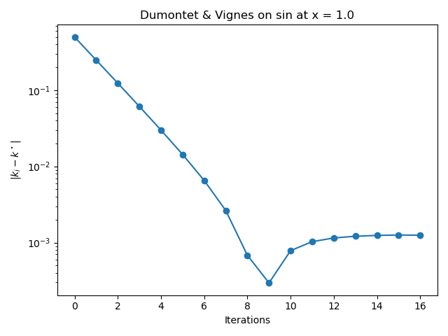
The previous figure shows that the algorithm gets closer to the optimal value of the step k in the early iterations. In the last iterations of the algorithm, the absolute error does not continue to decrease monotically and produces a final absolute error close to \(10^{-3}\).
Total running time of the script: (0 minutes 1.940 seconds)