Experiment with Stepleman & Winarsky method

Find a step which is near to optimal for a central finite difference formula.

References

• Adaptive numerical differentiation R. S. Stepleman and N. D. Winarsky Journal: Math. Comp. 33 (1979), 1257-1264

import numpy as np
import pylab as pl
import numericalderivative as nd
from matplotlib.ticker import MaxNLocator

Use the method on a simple problem

In the next example, we use the algorithm on the exponential function. We create the SteplemanWinarsky algorithm using the function and the point x. Then we use the find_step() method to compute the step, using an upper bound of the step as an initial point of the algorithm. Finally, use the compute_first_derivative() method to compute an approximate value of the first derivative using finite differences. The get_number_of_function_evaluations() method can be used to get the number of function evaluations.

x = 1.0
algorithm = nd.SteplemanWinarsky(np.exp, x, verbose=True)
initial_step = 1.0e0
step, number_of_iterations = algorithm.find_step(initial_step)
f_prime_approx = algorithm.compute_first_derivative(step)
feval = algorithm.get_number_of_function_evaluations()
f_prime_exact = np.exp(x)  # Since the derivative of exp is exp.
print(f"Computed step = {step:.3e}")
print(f"Number of number_of_iterations = {number_of_iterations}")
print(f"f_prime_approx = {f_prime_approx}")
print(f"f_prime_exact = {f_prime_exact}")
absolute_error = abs(f_prime_approx - f_prime_exact)

+ find_step()
initial_step=1.000e+00
  number_of_iterations=0, h=2.5000e-01, |FD(h_current) - FD(h_previous)|=4.4784e-01
  number_of_iterations=1, h=6.2500e-02, |FD(h_current) - FD(h_previous)|=2.6634e-02
  number_of_iterations=2, h=1.5625e-02, |FD(h_current) - FD(h_previous)|=1.6595e-03
  number_of_iterations=3, h=3.9062e-03, |FD(h_current) - FD(h_previous)|=1.0370e-04
  number_of_iterations=4, h=9.7656e-04, |FD(h_current) - FD(h_previous)|=6.4809e-06
  number_of_iterations=5, h=2.4414e-04, |FD(h_current) - FD(h_previous)|=4.0506e-07
  number_of_iterations=6, h=6.1035e-05, |FD(h_current) - FD(h_previous)|=2.5315e-08
  number_of_iterations=7, h=1.5259e-05, |FD(h_current) - FD(h_previous)|=1.5825e-09
  number_of_iterations=8, h=3.8147e-06, |FD(h_current) - FD(h_previous)|=1.1642e-10
  number_of_iterations=9, h=9.5367e-07, |FD(h_current) - FD(h_previous)|=1.1642e-10
  number_of_iterations=10, h=2.3842e-07, |FD(h_current) - FD(h_previous)|=4.6566e-10
  Stop because no monotony anymore.
Computed step = 9.537e-07
Number of number_of_iterations = 10
f_prime_approx = 2.7182818283326924
f_prime_exact = 2.718281828459045

Use the method on the ScaledExponentialProblem

Consider this problem.

problem = nd.ScaledExponentialProblem()
problem

DerivativeBenchmarkProblem

• name = scaled exp
• x = 1.0
• f(x) = 0.9999990000005
• f'(x) = -9.999990000004999e-07
• f''(x) = 9.999990000005e-13
• f^(3)(x) = -9.999990000005e-19
• f^(4)(x) = 9.999990000004998e-25
• f^(5)(x) = -9.999990000004998e-31

name = problem.get_name()
x = problem.get_x()
third_derivative = problem.get_third_derivative()
third_derivative_value = third_derivative(x)
optimum_step, absolute_error = nd.FirstDerivativeCentral.compute_step(
    third_derivative_value
)
print(f"Name = {name}, x = {x}")
print(f"Optimal step for central finite difference formula = {optimum_step}")
print(f"Minimum absolute error= {absolute_error}")

Name = scaled exp, x = 1.0
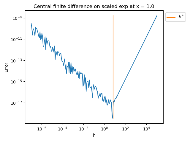
Optimal step for central finite difference formula = 6.694331732265233
Minimum absolute error= 2.2407016263779204e-17

Plot the error vs h

x = problem.get_x()
function = problem.get_function()
first_derivative = problem.get_first_derivative()
finite_difference = nd.FirstDerivativeCentral(function, x)
number_of_points = 200
step_array = np.logspace(-7.0, 5.0, number_of_points)
error_array = np.zeros((number_of_points))
for i in range(number_of_points):
    f_prime_approx = finite_difference.compute(step_array[i])
    error_array[i] = abs(f_prime_approx - first_derivative(x))

pl.figure()
pl.plot(step_array, error_array)
pl.plot([optimum_step] * 2, [min(error_array), max(error_array)], label=r"$h^*$")
pl.title(f"Central finite difference on {problem.get_name()} at x = {problem.get_x()}")
pl.xlabel("h")
pl.ylabel("Error")
pl.xscale("log")
pl.yscale("log")
pl.legend(bbox_to_anchor=(1, 1))
pl.tight_layout()

Use the algorithm to detect h*

function = problem.get_function()
first_derivative = problem.get_first_derivative()
algorithm = nd.SteplemanWinarsky(function, x, verbose=True)
initial_step = 1.0e8
x = problem.get_x()
h_optimal, number_of_iterations = algorithm.find_step(initial_step)
number_of_function_evaluations = algorithm.get_number_of_function_evaluations()
print("Optimum h =", h_optimal)
print("number_of_iterations =", number_of_iterations)
print("Function evaluations =", number_of_function_evaluations)
f_prime_approx = algorithm.compute_first_derivative(h_optimal)
absolute_error = abs(f_prime_approx - first_derivative(x))
print("Absolute error = ", absolute_error)

+ find_step()
initial_step=1.000e+08
  number_of_iterations=0, h=2.5000e+07, |FD(h_current) - FD(h_previous)|=1.3441e+35
  number_of_iterations=1, h=6.2500e+06, |FD(h_current) - FD(h_previous)|=1.4401e+03
  number_of_iterations=2, h=1.5625e+06, |FD(h_current) - FD(h_previous)|=3.9981e-05
  number_of_iterations=3, h=3.9062e+05, |FD(h_current) - FD(h_previous)|=4.3393e-07
  number_of_iterations=4, h=9.7656e+04, |FD(h_current) - FD(h_previous)|=2.4036e-08
  number_of_iterations=5, h=2.4414e+04, |FD(h_current) - FD(h_previous)|=1.4909e-09
  number_of_iterations=6, h=6.1035e+03, |FD(h_current) - FD(h_previous)|=9.3135e-11
  number_of_iterations=7, h=1.5259e+03, |FD(h_current) - FD(h_previous)|=5.8208e-12
  number_of_iterations=8, h=3.8147e+02, |FD(h_current) - FD(h_previous)|=3.6380e-13
  number_of_iterations=9, h=9.5367e+01, |FD(h_current) - FD(h_previous)|=2.2738e-14
  number_of_iterations=10, h=2.3842e+01, |FD(h_current) - FD(h_previous)|=1.4208e-15
  number_of_iterations=11, h=5.9605e+00, |FD(h_current) - FD(h_previous)|=8.3819e-17
  number_of_iterations=12, h=1.4901e+00, |FD(h_current) - FD(h_previous)|=9.3131e-18
  number_of_iterations=13, h=3.7253e-01, |FD(h_current) - FD(h_previous)|=3.7253e-17
  Stop because no monotony anymore.
Optimum h = 1.4901161193847656
number_of_iterations = 13
Function evaluations = 30
Absolute error =  1.9825229646960527e-17

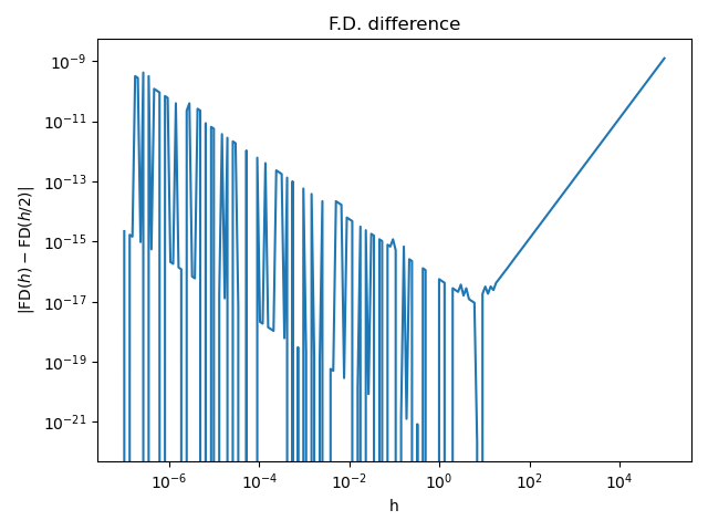
Plot the absolute difference depending on the step

def fd_difference(h1, h2, function, x):
    """
    Compute the difference of central difference approx. for different step sizes

    This function computes the absolute value of the difference of approximations
    evaluated at two different steps h1 and h2:

        d = abs(FD(h1) - FD(h2))

    where FD(h) is the approximation from the finite difference formula
    evaluated from the step h.

    Parameters
    ----------
    h1 : float, > 0
        The first step
    h2 : float, > 0
        The second step
    function : function
        The function
    x : float
        The input point where the derivative is approximated.
    """
    finite_difference = nd.FirstDerivativeCentral(function, x)
    f_prime_approx_1 = finite_difference.compute(h1)
    f_prime_approx_2 = finite_difference.compute(h2)
    diff_current = abs(f_prime_approx_1 - f_prime_approx_2)
    return diff_current

Plot the evolution of | FD(h) - FD(h / 2) | for different values of h

number_of_points = 200
step_array = np.logspace(-7.0, 5.0, number_of_points)
diff_array = np.zeros((number_of_points))
function = problem.get_function()
for i in range(number_of_points):
    diff_array[i] = fd_difference(step_array[i], step_array[i] / 2, function, x)

pl.figure()
pl.plot(step_array, diff_array)
pl.title("F.D. difference")
pl.xlabel("h")
pl.ylabel(r"$|\operatorname{FD}(h) - \operatorname{FD}(h / 2) |$")
pl.xscale("log")
pl.yscale("log")
pl.tight_layout()

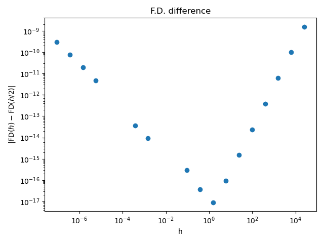
Plot the criterion depending on the step

Plot the evolution of | FD(h) - FD(h / 2) | for different values of h

number_of_points = 20
h_initial = 1.0e5
beta = 4.0
step_array = np.zeros((number_of_points))
diff_array = np.zeros((number_of_points))
function = problem.get_function()
for i in range(number_of_points):
    if i == 0:
        step_array[i] = h_initial / beta
        diff_array[i] = fd_difference(step_array[i], h_initial, function, x)
    else:
        step_array[i] = step_array[i - 1] / beta
        diff_array[i] = fd_difference(step_array[i], step_array[i - 1], function, x)

pl.figure()
pl.plot(step_array, diff_array, "o")
pl.title("F.D. difference")
pl.xlabel("h")
pl.ylabel(r"$|\operatorname{FD}(h) - \operatorname{FD}(h / 2) |$")
pl.xscale("log")
pl.yscale("log")
pl.tight_layout()

Compute reference step

p = 1.0e-16
beta = 4.0
h_reference = beta * p ** (1 / 3) * x
print("Suggested initial_step = ", h_reference)

Suggested initial_step =  1.8566355334451128e-05

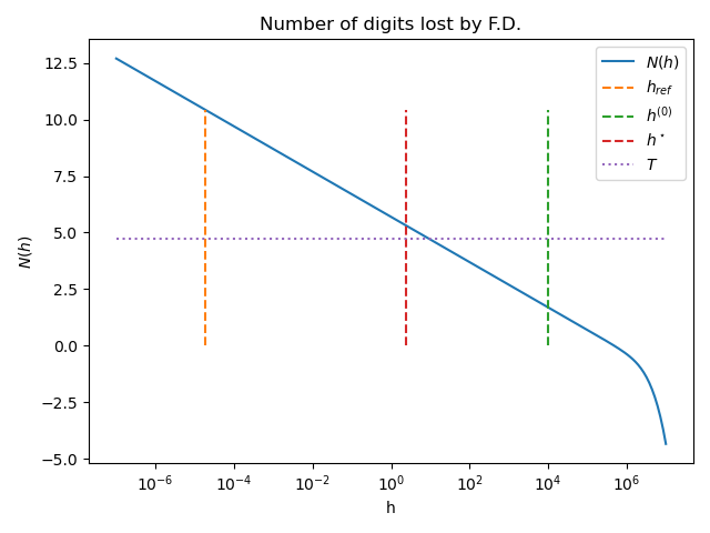
Plot number of lost digits vs h

The number_of_lost_digits() method computes the number of lost digits in the approximated derivative depending on the step.

h = 1.0e4
print("Starting h = ", h)
initialize = nd.SteplemanWinarskyInitialize(algorithm)
n_digits = initialize.number_of_lost_digits(h)
print("Number of lost digits = ", n_digits)
threshold = np.log10(p ** (-1.0 / 3.0) / beta)
print("Threshold = ", threshold)

initial_step, number_of_iterations = initialize.find_initial_step(
    1.0e-5,
    1.0e7,
)
print("initial_step = ", initial_step)
print("number_of_iterations = ", number_of_iterations)

estim_step, number_of_iterations = algorithm.find_step(initial_step)
print("estim_step = ", estim_step)
print("number_of_iterations = ", number_of_iterations)

Starting h =  10000.0
Number of lost digits =  1.6989627661187812
Threshold =  4.7312733420053705
initial_step =  10000.0
number_of_iterations =  1
+ find_step()
initial_step=1.000e+04
  number_of_iterations=0, h=2.5000e+03, |FD(h_current) - FD(h_previous)|=1.5625e-11
  number_of_iterations=1, h=6.2500e+02, |FD(h_current) - FD(h_previous)|=9.7656e-13
  number_of_iterations=2, h=1.5625e+02, |FD(h_current) - FD(h_previous)|=6.1035e-14
  number_of_iterations=3, h=3.9062e+01, |FD(h_current) - FD(h_previous)|=3.8142e-15
  number_of_iterations=4, h=9.7656e+00, |FD(h_current) - FD(h_previous)|=2.4016e-16
  number_of_iterations=5, h=2.4414e+00, |FD(h_current) - FD(h_previous)|=5.6844e-18
  number_of_iterations=6, h=6.1035e-01, |FD(h_current) - FD(h_previous)|=2.2737e-17
  Stop because no monotony anymore.
estim_step =  2.44140625
number_of_iterations =  6

number_of_points = 200
step_array = np.logspace(-7.0, 7.0, number_of_points)
n_digits_array = np.zeros((number_of_points))
for i in range(number_of_points):
    h = step_array[i]
    n_digits_array[i] = initialize.number_of_lost_digits(h)

y_max = initialize.number_of_lost_digits(h_reference)
pl.figure()
pl.plot(step_array, n_digits_array, label="$N(h)$")
pl.plot([h_reference] * 2, [0.0, y_max], "--", label=r"$h_{ref}$")
pl.plot([initial_step] * 2, [0.0, y_max], "--", label=r"$h^{(0)}$")
pl.plot([estim_step] * 2, [0.0, y_max], "--", label=r"$h^\star$")
pl.plot(
    step_array,
    np.array([threshold] * number_of_points),
    ":",
    label=r"$T$",
)
pl.title("Number of digits lost by F.D.")
pl.xlabel("h")
pl.ylabel("$N(h)$")
pl.xscale("log")
_ = pl.legend(bbox_to_anchor=(1.0, 1.0))
pl.tight_layout()

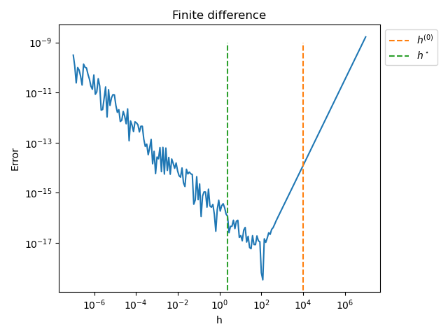
pl.figure()
pl.plot(step_array, error_array)
pl.plot([initial_step] * 2, [0.0, 1.0e-9], "--", label=r"$h^{(0)}$")
pl.plot([estim_step] * 2, [0.0, 1.0e-9], "--", label=r"$h^\star$")
pl.title("Finite difference")
pl.xlabel("h")
pl.ylabel("Error")
pl.xscale("log")
pl.legend(bbox_to_anchor=(1.0, 1.0))
pl.yscale("log")
pl.tight_layout()

Use the bisection search

In some cases, it is difficult to find the initial step. In this case, we can use the bisection algorithm, which can produce an initial guess for the step.c This algorithm is based on a search for a suitable step within an interval.

Test with single point and default parameters.

initialize = nd.SteplemanWinarskyInitialize(algorithm, relative_precision=1.0e-10)
initial_step, number_of_iterations = initialize.find_initial_step(
    1.0e-7,
    1.0e7,
)
feval = algorithm.get_number_of_function_evaluations()
print("initial_step = ", initial_step)
print("number_of_iterations = ", number_of_iterations)
print("Func. eval = ", feval)

initial_step =  3162.2776601683795
number_of_iterations =  1
Func. eval =  468

See how the algorithm behaves if we use or do not use the log scale when searching for the optimal step (this can be slower).

initialize = nd.SteplemanWinarskyInitialize(
    algorithm, relative_precision=1.0e-10, verbose=True
)
maximum_bisection = 53
print("+ No log scale.")
initial_step, number_of_iterations = initialize.find_initial_step(
    1.0e-7,
    1.0e8,
    maximum_bisection=maximum_bisection,
    log_scale=False,
)
print(
    f"Pas initial = {initial_step:.3e}, number_of_iterations = {number_of_iterations}"
)
print("+ Log scale.")

+ No log scale.
+ find_initial_step()
+ h_min = 1.000e-07, h_max = 1.000e+08
+ relative_precision = 1.000e-10
Searching for h such that 0 < N(h) <= n_treshold = 2.731
n_min = 12.699, n_max = -43.429
+ Iter 0 / 53, h_min = 1.000e-07, h_max = 1.000e+08
  h = 5.000e+07,   Number of lost digits = -21.715
  h is too large: reduce it
+ Iter 1 / 53, h_min = 1.000e-07, h_max = 5.000e+07
  h = 2.500e+07,   Number of lost digits = -10.857
  h is too large: reduce it
+ Iter 2 / 53, h_min = 1.000e-07, h_max = 2.500e+07
  h = 1.250e+07,   Number of lost digits = -5.429
  h is too large: reduce it
+ Iter 3 / 53, h_min = 1.000e-07, h_max = 1.250e+07
  h = 6.250e+06,   Number of lost digits = -2.714
  h is too large: reduce it
+ Iter 4 / 53, h_min = 1.000e-07, h_max = 6.250e+06
  h = 3.125e+06,   Number of lost digits = -1.356
  h is too large: reduce it
+ Iter 5 / 53, h_min = 1.000e-07, h_max = 3.125e+06
  h = 1.563e+06,   Number of lost digits = -0.659
  h is too large: reduce it
+ Iter 6 / 53, h_min = 1.000e-07, h_max = 1.563e+06
  h = 7.813e+05,   Number of lost digits = -0.237
  h is too large: reduce it
+ Iter 7 / 53, h_min = 1.000e-07, h_max = 7.813e+05
  h = 3.906e+05,   Number of lost digits = 0.096
  h is just right : stop !
Pas initial = 3.906e+05, number_of_iterations = 7
+ Log scale.

initial_step, number_of_iterations = initialize.find_initial_step(
    1.0e-7,
    1.0e8,
    maximum_bisection=maximum_bisection,
    log_scale=True,
)
print(
    f"Pas initial = {initial_step:.3e}, number_of_iterations = {number_of_iterations}"
)

+ find_initial_step()
+ h_min = 1.000e-07, h_max = 1.000e+08
+ relative_precision = 1.000e-10
Searching for h such that 0 < N(h) <= n_treshold = 2.731
n_min = 12.699, n_max = -43.429
+ Iter 0 / 53, h_min = 1.000e-07, h_max = 1.000e+08
  h = 3.162e+00,   Number of lost digits = 5.199
  h is small: increase it
+ Iter 1 / 53, h_min = 3.162e+00, h_max = 1.000e+08
  h = 1.778e+04,   Number of lost digits = 1.449
  h is just right : stop !
Pas initial = 1.778e+04, number_of_iterations = 1

In the next example, we search for an initial step using bisection, then use this step as an initial guess for the algorithm. Finally, we compute an approximation of the first derivative using the finite difference formula.

problem = nd.ExponentialProblem()
function = problem.get_function()
first_derivative = problem.get_first_derivative()
x = 1.0
algorithm = nd.SteplemanWinarsky(function, x, verbose=True)
initialize = nd.SteplemanWinarskyInitialize(algorithm)
initial_step, estim_relative_error = initialize.find_initial_step(
    1.0e-6,
    100.0 * x,
)
step, number_of_iterations = algorithm.find_step(initial_step)
f_prime_approx = algorithm.compute_first_derivative(step)
absolute_error = abs(f_prime_approx - first_derivative(x))
feval = algorithm.get_number_of_function_evaluations()
print(
    "x = %.3f, abs. error = %.3e, estim. rel. error = %.3e, Func. eval. = %d"
    % (x, absolute_error, estim_relative_error, number_of_function_evaluations)
)

+ find_step()
initial_step=1.000e-02
  number_of_iterations=0, h=2.5000e-03, |FD(h_current) - FD(h_previous)|=4.2473e-05
  number_of_iterations=1, h=6.2500e-04, |FD(h_current) - FD(h_previous)|=2.6546e-06
  number_of_iterations=2, h=1.5625e-04, |FD(h_current) - FD(h_previous)|=1.6591e-07
  number_of_iterations=3, h=3.9063e-05, |FD(h_current) - FD(h_previous)|=1.0366e-08
  number_of_iterations=4, h=9.7656e-06, |FD(h_current) - FD(h_previous)|=6.3665e-10
  number_of_iterations=5, h=2.4414e-06, |FD(h_current) - FD(h_previous)|=6.4055e-12
  number_of_iterations=6, h=6.1035e-07, |FD(h_current) - FD(h_previous)|=3.2409e-10
  Stop because no monotony anymore.
x = 1.000, abs. error = 6.533e-11, estim. rel. error = 0.000e+00, Func. eval. = 30

See the history of steps during the search

In Stepleman & Winarsky's method, the algorithm produces a sequence of steps \((h_i)_{1 \leq i \leq n_{iter}}\) where \(n_{iter} \in \mathbb{N}\) is the number of number_of_iterations. These steps are meant to converge to an approximately optimal step of for the central finite difference formula of the first derivative. The optimal step \(h^\star\) for the central finite difference formula of the first derivative can be computed depending on the third derivative of the function. In the next example, we want to compute the absolute error between each intermediate step \(h_i\) and the exact value \(h^\star\) to see how close the algorithm gets to the exact step. The list of intermediate steps during the algorithm can be obtained thanks to the get_step_history() method.

In the next example, we print the intermediate steps k during the bissection algorithm that searches for a step such that the L ratio is satisfactory.

problem = nd.SinProblem()
function = problem.get_function()
name = problem.get_name()
x = problem.get_x()
algorithm = nd.SteplemanWinarsky(function, x, verbose=True)
initial_step = 1.0e0
step, number_of_iterations = algorithm.find_step(initial_step)
step_h_history = algorithm.get_step_history()
print(f"Number of number_of_iterations = {number_of_iterations}")
print(f"History of steps h : {step_h_history}")
# The last step is not the best one, sinces it breaks the monotony
last_step_h = step_h_history[-2]
print(f"Last step h : {last_step_h}")

+ find_step()
initial_step=1.000e+00
  number_of_iterations=0, h=2.5000e-01, |FD(h_current) - FD(h_previous)|=8.0043e-02
  number_of_iterations=1, h=6.2500e-02, |FD(h_current) - FD(h_previous)|=5.2589e-03
  number_of_iterations=2, h=1.5625e-02, |FD(h_current) - FD(h_previous)|=3.2971e-04
  number_of_iterations=3, h=3.9062e-03, |FD(h_current) - FD(h_previous)|=2.0611e-05
  number_of_iterations=4, h=9.7656e-04, |FD(h_current) - FD(h_previous)|=1.2882e-06
  number_of_iterations=5, h=2.4414e-04, |FD(h_current) - FD(h_previous)|=8.0511e-08
  number_of_iterations=6, h=6.1035e-05, |FD(h_current) - FD(h_previous)|=5.0316e-09
  number_of_iterations=7, h=1.5259e-05, |FD(h_current) - FD(h_previous)|=3.1378e-10
  number_of_iterations=8, h=3.8147e-06, |FD(h_current) - FD(h_previous)|=2.9104e-11
  number_of_iterations=9, h=9.5367e-07, |FD(h_current) - FD(h_previous)|=1.4552e-11
  number_of_iterations=10, h=2.3842e-07, |FD(h_current) - FD(h_previous)|=1.7462e-10
  Stop because no monotony anymore.
Number of number_of_iterations = 10
History of steps h : [1.0, 0.25, 0.0625, 0.015625, 0.00390625, 0.0009765625, 0.000244140625, 6.103515625e-05, 1.52587890625e-05, 3.814697265625e-06, 9.5367431640625e-07, 2.384185791015625e-07]
Last step h : 9.5367431640625e-07

Then we compute the exact step, using find_step().

third_derivative = problem.get_third_derivative()
third_derivative_value = third_derivative(x)
print(f"f^(3)(x) = {third_derivative_value}")
absolute_precision = 1.0e-16
exact_step_k, absolute_error = nd.FirstDerivativeCentral.compute_step(
    third_derivative_value, absolute_precision
)
print(f"Optimal step k for f^(3)(x) = {exact_step_k}")

f^(3)(x) = -0.5403023058681398
Optimal step k for f^(3)(x) = 8.219173432436798e-06

Plot the absolute error between the exact step k and the intermediate k of the algorithm.

error_step_h = [
    abs(step_h_history[i] - exact_step_k) for i in range(len(step_h_history))
]
fig = pl.figure()
pl.title(f"Stepleman & Winarsky on {name} at x = {x}")
pl.plot(range(len(step_h_history)), error_step_h, "o-")
pl.xlabel("Iterations")
pl.ylabel(r"$|h_i - h^\star|$")
pl.yscale("log")
ax = fig.gca()
ax.xaxis.set_major_locator(MaxNLocator(integer=True))
pl.tight_layout()

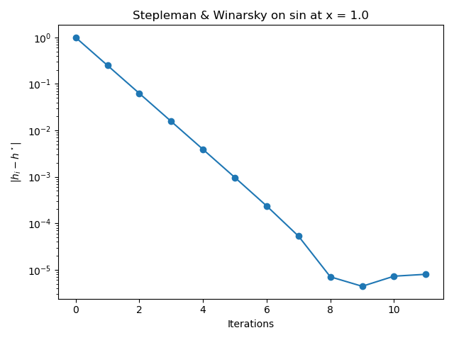
The previous figure shows that the algorithm gets closer to the optimal value of the step k in the early number_of_iterations. In the last number_of_iterations of the algorithm, the absolute error does not continue to decrease monotically and produces a final absolute error close to \(10^{-3}\).