Experiment with Shi, Xie, Xuan & Nocedal forward method

Find a step which is near to optimal for a forward finite difference formula.

References

• Shi, H. J. M., Xie, Y., Xuan, M. Q., & Nocedal, J. (2022). Adaptive finite-difference interval estimation for noisy derivative-free optimization. SIAM Journal on Scientific Computing, 44 (4), A2302-A2321.

import numpy as np
import pylab as pl
import numericalderivative as nd
from matplotlib.ticker import MaxNLocator

Use the method on a simple problem

In the next example, we use the algorithm on the exponential function. We create the ShiXieXuanNocedalForward algorithm using the function and the point x. Then we use the find_step() method to compute the step, using an upper bound of the step as an initial point of the algorithm. Finally, use the compute_first_derivative() method to compute an approximate value of the first derivative using finite differences. The get_number_of_function_evaluations() method can be used to get the number of function evaluations.

x = 1.0
algorithm = nd.ShiXieXuanNocedalForward(np.exp, x, verbose=True)
initial_step = 1.0
step, number_of_iterations = algorithm.find_step(initial_step)
f_prime_approx = algorithm.compute_first_derivative(step)
feval = algorithm.get_number_of_function_evaluations()
f_prime_exact = np.exp(x)  # Since the derivative of exp is exp.
print(f"Computed step = {step:.3e}")
print(f"Number of iterations = {number_of_iterations}")
print(f"f_prime_approx = {f_prime_approx}")
print(f"f_prime_exact = {f_prime_exact}")
absolute_error = abs(f_prime_approx - f_prime_exact)

x = 1.0
f(x) = 2.718281828459045
f(x + h) = 7.38905609893065
f(x + 4 * h) = 148.4131591025766
absolute_precision = 1.000e-15
estim_step=1.000e+00
+ Iter.=0, lower_bound=0.000e+00, upper_bound=inf, estim_step=1.000e+00, r = 1.588e+16
    - test_ratio > self.minimum_test_ratio. Set upper bound to h.
    - lower_bound == 0: decrease h.
+ Iter.=1, lower_bound=0.000e+00, upper_bound=1.000e+00, estim_step=2.500e-01, r = 1.978e+14
    - test_ratio > self.minimum_test_ratio. Set upper bound to h.
    - lower_bound == 0: decrease h.
+ Iter.=2, lower_bound=0.000e+00, upper_bound=2.500e-01, estim_step=6.250e-02, r = 8.851e+12
    - test_ratio > self.minimum_test_ratio. Set upper bound to h.
    - lower_bound == 0: decrease h.
+ Iter.=3, lower_bound=0.000e+00, upper_bound=6.250e-02, estim_step=1.562e-02, r = 5.109e+11
    - test_ratio > self.minimum_test_ratio. Set upper bound to h.
    - lower_bound == 0: decrease h.
+ Iter.=4, lower_bound=0.000e+00, upper_bound=1.562e-02, estim_step=3.906e-03, r = 3.131e+10
    - test_ratio > self.minimum_test_ratio. Set upper bound to h.
    - lower_bound == 0: decrease h.
+ Iter.=5, lower_bound=0.000e+00, upper_bound=3.906e-03, estim_step=9.766e-04, r = 1.947e+09
    - test_ratio > self.minimum_test_ratio. Set upper bound to h.
    - lower_bound == 0: decrease h.
+ Iter.=6, lower_bound=0.000e+00, upper_bound=9.766e-04, estim_step=2.441e-04, r = 1.216e+08
    - test_ratio > self.minimum_test_ratio. Set upper bound to h.
    - lower_bound == 0: decrease h.
+ Iter.=7, lower_bound=0.000e+00, upper_bound=2.441e-04, estim_step=6.104e-05, r = 7.596e+06
    - test_ratio > self.minimum_test_ratio. Set upper bound to h.
    - lower_bound == 0: decrease h.
+ Iter.=8, lower_bound=0.000e+00, upper_bound=6.104e-05, estim_step=1.526e-05, r = 4.747e+05
    - test_ratio > self.minimum_test_ratio. Set upper bound to h.
    - lower_bound == 0: decrease h.
+ Iter.=9, lower_bound=0.000e+00, upper_bound=1.526e-05, estim_step=3.815e-06, r = 2.967e+04
    - test_ratio > self.minimum_test_ratio. Set upper bound to h.
    - lower_bound == 0: decrease h.
+ Iter.=10, lower_bound=0.000e+00, upper_bound=3.815e-06, estim_step=9.537e-07, r = 1.854e+03
    - test_ratio > self.minimum_test_ratio. Set upper bound to h.
    - lower_bound == 0: decrease h.
+ Iter.=11, lower_bound=0.000e+00, upper_bound=9.537e-07, estim_step=2.384e-07, r = 1.157e+02
    - test_ratio > self.minimum_test_ratio. Set upper bound to h.
    - lower_bound == 0: decrease h.
+ Iter.=12, lower_bound=0.000e+00, upper_bound=2.384e-07, estim_step=5.960e-08, r = 7.327e+00
    - test_ratio > self.minimum_test_ratio. Set upper bound to h.
    - lower_bound == 0: decrease h.
+ Iter.=13, lower_bound=0.000e+00, upper_bound=5.960e-08, estim_step=1.490e-08, r = 4.441e-01
    - test_ratio < self.minimum_test_ratio. Set lower bound to h.
    - Bisection: estim_step = 2.980e-08.
+ Iter.=14, lower_bound=1.490e-08, upper_bound=5.960e-08, estim_step=2.980e-08, r = 1.776e+00
    - Step = 2.9802322387695405e-08 is OK: stop.
Computed step = 2.980e-08
Number of iterations = 14
f_prime_approx = 2.7182818800210953
f_prime_exact = 2.718281828459045

Use the method on the ScaledExponentialProblem

Consider this problem.

problem = nd.ScaledExponentialProblem()
print(problem)
name = problem.get_name()
x = problem.get_x()
second_derivative = problem.get_second_derivative()
second_derivative_value = second_derivative(x)
optimum_step, absolute_error = nd.FirstDerivativeForward.compute_step(
    second_derivative_value
)
print(f"Name = {name}, x = {x}")
print(f"Optimal step for forward finite difference formula = {optimum_step}")
print(f"Minimum absolute error= {absolute_error}")

DerivativeBenchmarkProblem
name = scaled exp
x = 1.0
f(x) = 0.9999990000005
f'(x) = -9.999990000004999e-07
f''(x) = 9.999990000005e-13
f^(3)(x) = -9.999990000005e-19
f^(4)(x) = 9.999990000004998e-25
f^(5)(x) = -9.999990000004998e-31

Name = scaled exp, x = 1.0
Optimal step for forward finite difference formula = 0.0200000100000025
Minimum absolute error= 1.99999900000025e-14

Plot the error vs h

function = problem.get_function()
first_derivative = problem.get_first_derivative()
finite_difference = nd.FirstDerivativeForward(function, x)
number_of_points = 1000
step_array = np.logspace(-8.0, 4.0, number_of_points)
error_array = np.zeros((number_of_points))
for i in range(number_of_points):
    h = step_array[i]
    f_prime_approx = finite_difference.compute(h)
    error_array[i] = abs(f_prime_approx - first_derivative(x))

pl.figure()
pl.plot(step_array, error_array)
pl.plot([optimum_step] * 2, [min(error_array), max(error_array)], label=r"$h^*$")
pl.title("Forward finite difference")
pl.xlabel("h")
pl.ylabel("Error")
pl.xscale("log")
pl.yscale("log")
pl.legend(bbox_to_anchor=(1, 1))
pl.tight_layout()

Use the algorithm to detect h*

algorithm = nd.ShiXieXuanNocedalForward(function, x, verbose=True)
x = 1.0e0
initial_step = 1.0
h_optimal, iterations = algorithm.find_step(initial_step)
number_of_function_evaluations = algorithm.get_number_of_function_evaluations()
print("Optimum h =", h_optimal)
print("iterations =", iterations)
print("Function evaluations =", number_of_function_evaluations)
f_prime_approx = algorithm.compute_first_derivative(h_optimal)
absolute_error = abs(f_prime_approx - problem.first_derivative(x))
print("Error = ", absolute_error)

x = 1.0
f(x) = 0.9999990000005
f(x + h) = 0.999998000002
f(x + 4 * h) = 0.9999950000125
absolute_precision = 1.000e-15
estim_step=1.000e+00
+ Iter.=0, lower_bound=0.000e+00, upper_bound=inf, estim_step=1.000e+00, r = 7.500e+02
    - test_ratio > self.minimum_test_ratio. Set upper bound to h.
    - lower_bound == 0: decrease h.
+ Iter.=1, lower_bound=0.000e+00, upper_bound=1.000e+00, estim_step=2.500e-01, r = 4.691e+01
    - test_ratio > self.minimum_test_ratio. Set upper bound to h.
    - lower_bound == 0: decrease h.
+ Iter.=2, lower_bound=0.000e+00, upper_bound=2.500e-01, estim_step=6.250e-02, r = 2.942e+00
    - Step = 0.0625 is OK: stop.
Optimum h = 0.0625
iterations = 2
Function evaluations = 5
Error =  3.1035867193208197e-14

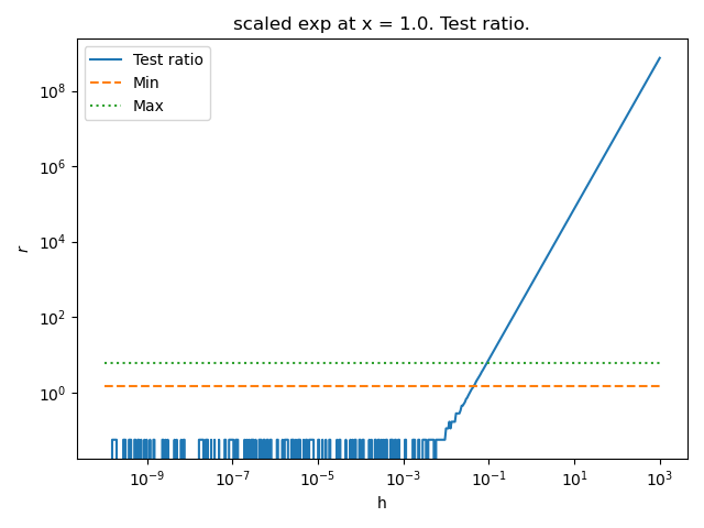
Plot the criterion depending on the step

Plot the test ratio depending on h

problem = nd.ScaledExponentialProblem()
function = problem.get_function()
name = problem.get_name()
x = problem.get_x()
algorithm = nd.ShiXieXuanNocedalForward(function, x, verbose=True)
minimum_test_ratio, maximum_test_ratio = algorithm.get_ratio_min_max()
absolute_precision = 1.0e-15
number_of_points = 500
step_array = np.logspace(-10.0, 3.0, number_of_points)
test_ratio_array = np.zeros((number_of_points))
for i in range(number_of_points):
    test_ratio_array[i] = algorithm.compute_test_ratio(
        step_array[i],
    )

pl.figure()
pl.plot(step_array, test_ratio_array, "-", label="Test ratio")
pl.plot(step_array, [minimum_test_ratio] * number_of_points, "--", label="Min")
pl.plot(step_array, [maximum_test_ratio] * number_of_points, ":", label="Max")
pl.title(f"{name} at x = {x}. Test ratio.")
pl.xlabel("h")
pl.ylabel(r"$r$")
pl.xscale("log")
pl.yscale("log")
pl.legend()
pl.tight_layout()

See the history of steps during the search

In Shi, Xie, Xuan & Nocedal's method, the algorithm produces a sequence of steps \((h_i)_{1 \leq i \leq n_{iter}}\) where \(n_{iter} \in \mathbb{N}\) is the number of iterations. These steps are meant to converge to an approximately optimal step of for the forward finite difference formula of the first derivative. The optimal step \(h^\star\) for the central finite difference formula of the first derivative can be computed depending on the second derivative of the function. In the next example, we want to compute the absolute error between each intermediate step \(h_i\) and the exact value \(h^\star\) to see how close the algorithm gets to the exact step. The list of intermediate steps during the algorithm can be obtained thanks to the get_step_history() method.

In the next example, we print the intermediate steps k during the bissection algorithm that searches for a step such that the L ratio is satisfactory.

problem = nd.ScaledExponentialProblem()
function = problem.get_function()
name = problem.get_name()
x = problem.get_x()
algorithm = nd.ShiXieXuanNocedalForward(function, x, verbose=True)
initial_step = 1.0e5
step, number_of_iterations = algorithm.find_step(initial_step)
step_h_history = algorithm.get_step_history()
print(f"Number of iterations = {number_of_iterations}")
print(f"History of steps h : {step_h_history}")
last_step_h = step_h_history[-1]
print(f"Last step h : {last_step_h}")

x = 1.0
f(x) = 0.9999990000005
f(x + h) = 0.9048365131989939
f(x + 4 * h) = 0.6703193757159285
absolute_precision = 1.000e-15
estim_step=1.000e+05
+ Iter.=0, lower_bound=0.000e+00, upper_bound=inf, estim_step=1.000e+05, r = 6.371e+12
    - test_ratio > self.minimum_test_ratio. Set upper bound to h.
    - lower_bound == 0: decrease h.
+ Iter.=1, lower_bound=0.000e+00, upper_bound=1.000e+05, estim_step=2.500e+04, r = 4.497e+11
    - test_ratio > self.minimum_test_ratio. Set upper bound to h.
    - lower_bound == 0: decrease h.
+ Iter.=2, lower_bound=0.000e+00, upper_bound=2.500e+04, estim_step=6.250e+03, r = 2.899e+10
    - test_ratio > self.minimum_test_ratio. Set upper bound to h.
    - lower_bound == 0: decrease h.
+ Iter.=3, lower_bound=0.000e+00, upper_bound=6.250e+03, estim_step=1.562e+03, r = 1.826e+09
    - test_ratio > self.minimum_test_ratio. Set upper bound to h.
    - lower_bound == 0: decrease h.
+ Iter.=4, lower_bound=0.000e+00, upper_bound=1.562e+03, estim_step=3.906e+02, r = 1.144e+08
    - test_ratio > self.minimum_test_ratio. Set upper bound to h.
    - lower_bound == 0: decrease h.
+ Iter.=5, lower_bound=0.000e+00, upper_bound=3.906e+02, estim_step=9.766e+01, r = 7.151e+06
    - test_ratio > self.minimum_test_ratio. Set upper bound to h.
    - lower_bound == 0: decrease h.
+ Iter.=6, lower_bound=0.000e+00, upper_bound=9.766e+01, estim_step=2.441e+01, r = 4.470e+05
    - test_ratio > self.minimum_test_ratio. Set upper bound to h.
    - lower_bound == 0: decrease h.
+ Iter.=7, lower_bound=0.000e+00, upper_bound=2.441e+01, estim_step=6.104e+00, r = 2.794e+04
    - test_ratio > self.minimum_test_ratio. Set upper bound to h.
    - lower_bound == 0: decrease h.
+ Iter.=8, lower_bound=0.000e+00, upper_bound=6.104e+00, estim_step=1.526e+00, r = 1.746e+03
    - test_ratio > self.minimum_test_ratio. Set upper bound to h.
    - lower_bound == 0: decrease h.
+ Iter.=9, lower_bound=0.000e+00, upper_bound=1.526e+00, estim_step=3.815e-01, r = 1.092e+02
    - test_ratio > self.minimum_test_ratio. Set upper bound to h.
    - lower_bound == 0: decrease h.
+ Iter.=10, lower_bound=0.000e+00, upper_bound=3.815e-01, estim_step=9.537e-02, r = 6.828e+00
    - test_ratio > self.minimum_test_ratio. Set upper bound to h.
    - lower_bound == 0: decrease h.
+ Iter.=11, lower_bound=0.000e+00, upper_bound=9.537e-02, estim_step=2.384e-02, r = 4.996e-01
    - test_ratio < self.minimum_test_ratio. Set lower bound to h.
    - Bisection: estim_step = 4.768e-02.
+ Iter.=12, lower_bound=2.384e-02, upper_bound=9.537e-02, estim_step=4.768e-02, r = 1.721e+00
    - Step = 0.04768371582031251 is OK: stop.
Number of iterations = 12
History of steps h : [100000.0, 25000.0, 6250.0, 1562.5, 390.625, 97.65625, 24.4140625, 6.103515625, 1.52587890625, 0.3814697265625, 0.095367431640625, 0.02384185791015625, np.float64(0.04768371582031251)]
Last step h : 0.04768371582031251

Then we compute the exact step, using compute_step().

second_derivative = problem.get_second_derivative()
second_derivative_value = second_derivative(x)
print(f"f^(2)(x) = {second_derivative_value}")
absolute_precision = 1.0e-16
exact_step, absolute_error = nd.FirstDerivativeForward.compute_step(
    second_derivative_value, absolute_precision
)
print(f"Optimal step k for f'(x) using forward F.D. = {exact_step}")

f^(2)(x) = 9.999990000005e-13
Optimal step k for f'(x) using forward F.D. = 0.0200000100000025

Plot the absolute error between the exact step k and the intermediate k of the algorithm.

error_step_h = [abs(step_h_history[i] - exact_step) for i in range(len(step_h_history))]
fig = pl.figure(figsize=(4.0, 3.0))
pl.title(f"Shi, Xie, Xuan & Nocedal on {name} at x = {x}")
pl.plot(range(len(step_h_history)), error_step_h, "o-")
pl.xlabel("Iterations")
pl.ylabel(r"$|h_i - h^\star|$")
pl.yscale("log")
ax = fig.gca()
ax.xaxis.set_major_locator(MaxNLocator(integer=True))
pl.tight_layout()

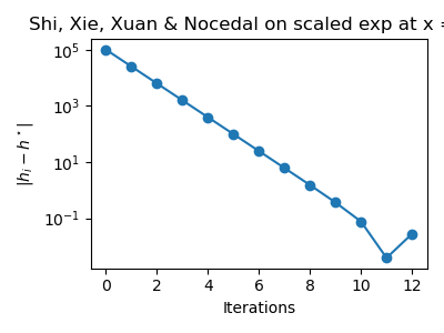
The previous figure shows that the algorithm converges relatively fast. The absolute error does not evolve monotically.