Experiment with Gill, Murray, Saunders and Wright method

Find a step which is near to optimal for a central finite difference formula.

References

• Gill, P. E., Murray, W., Saunders, M. A., & Wright, M. H. (1983). Computing forward-difference intervals for numerical optimization. SIAM Journal on Scientific and Statistical Computing, 4(2), 310-321.

import numpy as np
import pylab as pl
import numericalderivative as nd
from matplotlib.ticker import MaxNLocator

Use the method on a simple problem

In the next example, we use the algorithm on the exponential function. We create the GillMurraySaundersWright algorithm using the function and the point x. Then we use the find_step() method to compute the step, using an upper bound of the step as an initial point of the algorithm. Finally, use the compute_first_derivative() method to compute an approximate value of the first derivative using finite differences. The get_number_of_function_evaluations() method can be used to get the number of function evaluations.

x = 1.0
algorithm = nd.GillMurraySaundersWright(np.exp, x, verbose=True)
kmin = 1.0e-10
kmax = 1.0e0
step, number_of_iterations = algorithm.find_step(kmin, kmax)
f_prime_approx = algorithm.compute_first_derivative(step)
feval = algorithm.get_number_of_function_evaluations()
f_prime_exact = np.exp(x)  # Since the derivative of exp is exp.
print(f"Computed step = {step:.3e}")
print(f"Number of iterations = {number_of_iterations}")
print(f"f_prime_approx = {f_prime_approx}")
print(f"f_prime_exact = {f_prime_exact}")
absolute_error = abs(f_prime_approx - f_prime_exact)

kmin = 1.000e-10, c(kmin) = 9.007e+00
kmax = 1.000e+00, c(kmax) = 1.355e-15
Iter #0, kmin = 1.000e-10, kmax = 1.000e+00, k = 1.000e-05, c(k) = 1.472e-05
  c(k) < c_threshold_min: reduce kmax.
Iter #1, kmin = 1.000e-10, kmax = 1.000e-05, k = 3.162e-08, c(k) = 1.287e+00
  c(k) >= c_threshold_min: increase kmin.
Iter #2, kmin = 3.162e-08, kmax = 1.000e-05, k = 5.623e-07, c(k) = 4.650e-03
  c in [0.001, 0.1]: stop!
Computed step = 3.835e-08
Number of iterations = 2
f_prime_approx = 2.71828188987139
f_prime_exact = 2.718281828459045

Test the method on the exponential problem

The next function is an oracle which returns the absolute precision of the value of the function.

def absolute_precision_oracle(function, x, relative_precision):
    """
    Return the absolute precision of the function value

    This oracle may fail if the function value is zero.

    Parameters
    ----------
    function : function
        The function
    x : float
        The test point
    relative_precision : float, > 0, optional
        The relative precision of evaluation of f.

    Returns
    -------
    absolute_precision : float, >= 0
        The absolute precision
    """
    function_value = function(x)
    if function_value == 0.0:
        raise ValueError(
            "The function value is zero: " "cannot compute the absolute precision"
        )
    absolute_precision = relative_precision * abs(function_value)
    return absolute_precision

class GillMurraySaundersWrightMethod:
    def __init__(self, kmin, kmax, relative_precision):
        """
        Create a GillMurraySaundersWright method to compute the approximate first derivative

        Parameters
        ----------
        kmin : float, kmin > 0
            A minimum bound for the finite difference step of the third derivative.
            If no value is provided, the default is to compute the smallest
            possible kmin using number_of_digits and x.
        kmax : float, kmax > kmin > 0
            A maximum bound for the finite difference step of the third derivative.
            If no value is provided, the default is to compute the largest
            possible kmax using number_of_digits and x.
        relative_precision : float, > 0, optional
            The relative precision of evaluation of f.
        """
        self.kmin = kmin
        self.kmax = kmax
        self.relative_precision = relative_precision

    def compute_first_derivative(self, function, x):
        """
        Compute the first derivative using GillMurraySaundersWright

        Parameters
        ----------
        function : function
            The function
        x : float
            The test point

        Returns
        -------
        f_prime_approx : float
            The approximate value of the first derivative of the function at point x
        number_of_function_evaluations : int
            The number of function evaluations.
        """
        absolute_precision = absolute_precision_oracle(
            function, x, self.relative_precision
        )
        algorithm = nd.GillMurraySaundersWright(
            function, x, absolute_precision=absolute_precision
        )
        step, _ = algorithm.find_step(kmin, kmax)
        f_prime_approx = algorithm.compute_first_derivative(step)
        number_of_function_evaluations = algorithm.get_number_of_function_evaluations()
        return f_prime_approx, number_of_function_evaluations

def compute_first_derivative_GMSW(
    function,
    x,
    first_derivative,
    kmin,
    kmax,
    relative_precision=1.0e-15,
    verbose=False,
):
    """
    Compute the approximate derivative from finite differences

    Parameters
    ----------
    function : function
        The function.
    x : float
        The point where the derivative is to be evaluated
    first_derivative : function
        The exact first derivative of the function.
    kmin : float, > 0
        The minimum step k for the second derivative.
    kmax : float, > kmin
        The maximum step k for the second derivative.
    relative_precision : float, > 0, optional
        The relative precision of evaluation of f.
    verbose : bool, optional
        Set to True to print intermediate messages. The default is False.

    Returns
    -------
    relative_error : float, > 0
        The relative error between the approximate first derivative
        and the true first derivative.

    feval : int
        The number of function evaluations.
    """

    method = GillMurraySaundersWrightMethod(kmin, kmax, relative_precision)
    f_prime_approx, number_of_function_evaluations = method.compute_first_derivative(
        function, x
    )
    f_prime_exact = first_derivative(x)
    if verbose:
        print(f"Computed step = {step:.3e}")
        print(f"Number of iterations = {number_of_iterations}")
        print(f"f_prime_approx = {f_prime_approx}")
        print(f"f_prime_exact = {f_prime_exact}")
    absolute_error = abs(f_prime_approx - f_prime_exact)
    return absolute_error, number_of_function_evaluations

print("+ Test on ExponentialProblem")
kmin = 1.0e-15
kmax = 1.0e1
x = 1.0
problem = nd.ExponentialProblem()
problem

+ Test on ExponentialProblem

DerivativeBenchmarkProblem

• name = exp
• x = 1.0
• f(x) = 2.718281828459045
• f'(x) = 2.718281828459045
• f''(x) = 2.718281828459045
• f^(3)(x) = 2.718281828459045
• f^(4)(x) = 2.718281828459045
• f^(5)(x) = 2.718281828459045

second_derivative_value = problem.second_derivative(x)
optimal_step, absolute_error = nd.FirstDerivativeForward.compute_step(
    second_derivative_value
)
print("Exact h* = %.3e" % (optimal_step))
(
    absolute_error,
    number_of_function_evaluations,
) = compute_first_derivative_GMSW(
    problem.function,
    x,
    problem.first_derivative,
    kmin,
    kmax,
    verbose=True,
)
print(
    "x = %.3f, error = %.3e, Func. eval. = %d"
    % (x, absolute_error, number_of_function_evaluations)
)

Exact h* = 1.213e-08
Computed step = 3.835e-08
Number of iterations = 2
f_prime_approx = 2.7182819133272096
f_prime_exact = 2.718281828459045
x = 1.000, error = 8.487e-08, Func. eval. = 18

print("+ Test on ScaledExponentialDerivativeBenchmark")
kmin = 1.0e-9
kmax = 1.0e8
x = 1.0
problem = nd.ScaledExponentialProblem()
second_derivative = problem.get_second_derivative()
second_derivative_value = second_derivative(x)
optimal_step, absolute_error = nd.FirstDerivativeForward.compute_step(
    second_derivative_value
)
print("Exact h* = %.3e" % (optimal_step))
(
    absolute_error,
    number_of_function_evaluations,
) = compute_first_derivative_GMSW(
    problem.get_function(),
    x,
    problem.get_first_derivative(),
    kmin,
    kmax,
    verbose=True,
)
print(
    "x = %.3f, error = %.3e, Func. eval. = %d"
    % (x, absolute_error, number_of_function_evaluations)
)

+ Test on ScaledExponentialDerivativeBenchmark
Exact h* = 2.000e-02
Computed step = 3.835e-08
Number of iterations = 2
f_prime_approx = -9.999989687168326e-07
f_prime_exact = -9.999990000004999e-07
x = 1.000, error = 3.128e-14, Func. eval. = 12

Benchmark the method on a collection of test points

print("+ Benchmark on several points on ScaledExponentialProblem")
number_of_test_points = 100
problem = nd.ScaledExponentialProblem()
interval = problem.get_interval()
test_points = np.linspace(interval[0], interval[1], number_of_test_points)
kmin = 1.0e-12
kmax = 1.0e1
relative_precision = 1.0e-15
method = GillMurraySaundersWrightMethod(kmin, kmax, relative_precision)
average_error, average_feval, _ = nd.benchmark_method(
    problem.get_function(),
    problem.get_fifth_derivative(),
    test_points,
    method.compute_first_derivative,
    False,
)
print("Average error =", average_error)
print("Average number of function evaluations =", average_feval)

+ Benchmark on several points on ScaledExponentialProblem
Average error = 9.999999683394813e+23
Average number of function evaluations = 16.0

Plot the condition error depending on the step

def plot_condition_error(name, function, x, kmin, kmax, number_of_points=1000):
    # Plot the condition error depending on k.
    k_array = np.logspace(np.log10(kmin), np.log10(kmax), number_of_points)
    algorithm = nd.GillMurraySaundersWright(function, x)
    c_min, c_max = algorithm.get_threshold_min_max()
    condition_array = np.zeros((number_of_points))
    for i in range(number_of_points):
        condition_array[i] = algorithm.compute_condition(k_array[i])

    #
    pl.figure()
    pl.title(f"Condition error of {name} at x = {x}")
    pl.plot(k_array, condition_array)
    pl.plot([kmin, kmax], [c_min] * 2, label=r"$c_{min}$")
    pl.plot([kmin, kmax], [c_max] * 2, label=r"$c_{max}$")
    pl.xlabel(r"$h_\Phi$")
    pl.ylabel(r"$c(h_\Phi$)")
    pl.xscale("log")
    pl.yscale("log")
    pl.legend(bbox_to_anchor=(1.0, 1.0))
    pl.tight_layout()
    return

The next plot presents the condition error \(c(h_\Phi)\) depending on \(h_\Phi\). The two horizontal lines represent the minimum and maximum threshold values. We search for the value of \(h_\Phi\) such that the condition error is between these two limits.

number_of_points = 200
problem = nd.ScaledExponentialProblem()
x = problem.get_x()
name = problem.get_name()
function = problem.get_function()
kmin = 1.0e-10
kmax = 1.0e5
plot_condition_error(name, function, x, kmin, kmax)

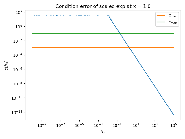
The previous plot shows that the condition error is a decreasing function of \(h_\Phi\).

Remove the end points \(x = \pm \pi\), because sin has a zero second derivative at these points. This makes the algorithm fail.

print("+ Benchmark on several points on SinProblem")
number_of_test_points = 100
problem = nd.SinProblem()
interval = problem.get_interval()
epsilon = 1.0e-3
test_points = np.linspace(
    interval[0] + epsilon, interval[1] - epsilon, number_of_test_points
)
kmin = 1.0e-12
kmax = 1.0e1
relative_precision = 1.0e-15
method = GillMurraySaundersWrightMethod(kmin, kmax, relative_precision)
average_error, average_feval, _ = nd.benchmark_method(
    problem.get_function(),
    problem.get_fifth_derivative(),
    test_points,
    method.compute_first_derivative,
    False,
)
print("Average error =", average_error)
print("Average number of function evaluations =", average_feval)

+ Benchmark on several points on SinProblem
Average error = 1.0720752779539923e-07
Average number of function evaluations = 18.0

Plot the condition error depending on k.

number_of_points = 200
problem = nd.SinProblem()
x = -np.pi
name = problem.get_name()
function = problem.get_function()
kmin = 1.0e-17
kmax = 1.0e-10
plot_condition_error(name, function, x, kmin, kmax)

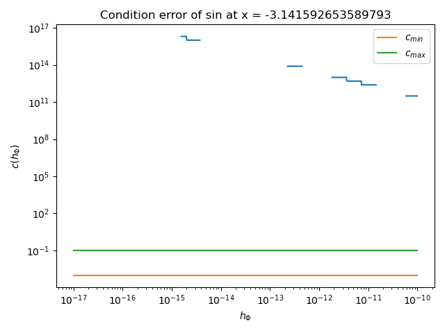
In the previous plot, we see that there is no satisfactory value of \(h_\Phi\) for the sin function at point \(x = -\pi\).

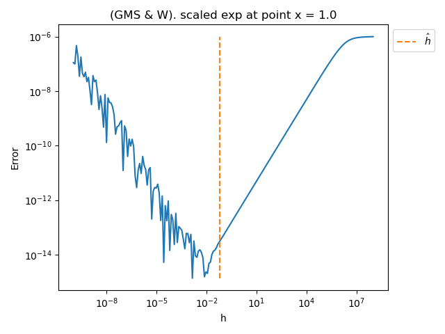
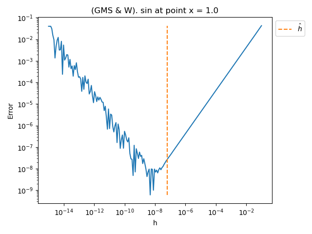
Plot the error depending on the step

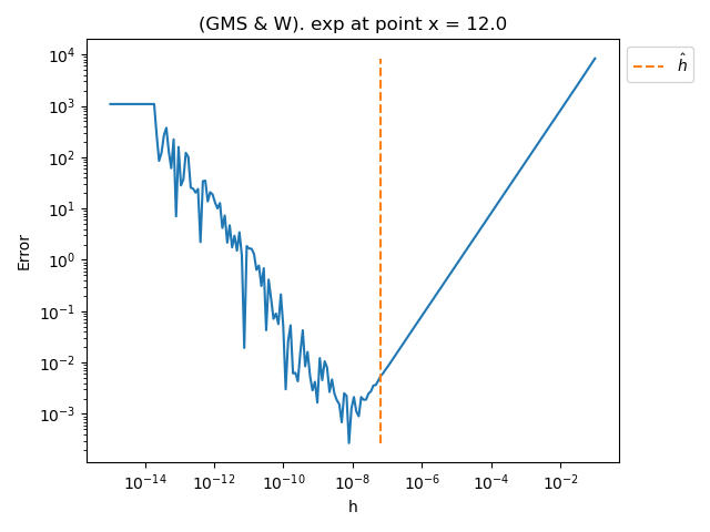
For each function, at point x = 1, plot the error vs the step computed by the method

def plot_error_vs_h_with_GMSW_steps(
    name,
    function,
    first_derivative,
    x,
    step_array,
    kmin,
    kmax,
    relative_precision=1.0e-15,
    verbose=False,
):
    """
    Plot the computed error depending on the step for an array of F.D. steps

    Parameters
    ----------
    name : str
        The name of the problem
    function : function
        The function.
    first_derivative : function
        The exact first derivative of the function
    x : float
        The input point where the test is done
    step_array : list(float)
        The array of finite difference steps
    kmin : float, > 0
        The minimum step k for the second derivative.
    kmax : float, > kmin
        The maximum step k for the second derivative.
    relative_precision : float, optional
        The relative precision of the function f at the point x.
    verbose : bool, optional
        Set to True to print intermediate messages. The default is False.
    """

    function_value = function(x)
    if function_value == 0.0:
        raise ValueError(
            "The function value is zero: cannot compute "
            "the absolute precision from the relative precision. "
            "Please set the absolute precision specifically."
        )
    absolute_precision = relative_precision * abs(function_value)
    algorithm = nd.GillMurraySaundersWright(function, x, absolute_precision)
    number_of_points = len(step_array)
    error_array = np.zeros((number_of_points))
    for i in range(number_of_points):
        f_prime_approx = algorithm.compute_first_derivative(step_array[i])
        error_array[i] = abs(f_prime_approx - first_derivative(x))

    step, number_of_iterations = algorithm.find_step(kmin, kmax)

    if verbose:
        print(name)
        print(f"Step h* = {step:.3e} using {number_of_iterations} iterations")

    minimum_error = np.nanmin(error_array)
    maximum_error = np.nanmax(error_array)

    pl.figure()
    pl.plot(step_array, error_array)
    pl.plot(
        [step] * 2,
        [minimum_error, maximum_error],
        "--",
        label=r"$\hat{h}$",
    )
    pl.title(f"(GMS & W). {name} at point x = {x}")
    pl.xlabel("h")
    pl.ylabel("Error")
    pl.xscale("log")
    pl.yscale("log")
    pl.legend(bbox_to_anchor=(1.0, 1.0))
    pl.tight_layout()
    return

def plot_error_vs_h_benchmark(
    problem, x, step_array, kmin, kmax, relative_precision=1.0e-15, verbose=False
):
    """
    Plot the computed error depending on the step for an array of F.D. steps

    Parameters
    ----------
    problem : nd.BenchmarkProblem
        The problem
    x : float
        The input point where the test is done
    step_array : list(float)
        The array of finite difference steps
    kmin : float, > 0
        The minimum step k for the second derivative.
    kmax : float, > kmin
        The maximum step k for the second derivative.
    relative_precision : float, optional
        The relative error of the function f at the point x.
    verbose : bool, optional
        Set to True to print intermediate messages. The default is False.
    """
    plot_error_vs_h_with_GMSW_steps(
        problem.get_name(),
        problem.get_function(),
        problem.get_first_derivative(),
        x,
        step_array,
        kmin,
        kmax,
        relative_precision,
        verbose,
    )

problem = nd.ExponentialProblem()
x = 1.0
number_of_points = 200
step_array = np.logspace(-15.0, -1.0, number_of_points)
kmin = 1.0e-15
kmax = 1.0e-1
relative_precision = 1.0e-15
plot_error_vs_h_benchmark(problem, x, step_array, kmin, kmax, relative_precision, True)

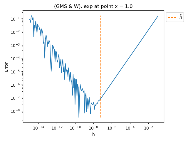
exp
Step h* = 6.322e-08 using 2 iterations

x = 12.0
step_array = np.logspace(-15.0, -1.0, number_of_points)
plot_error_vs_h_benchmark(problem, x, step_array, kmin, kmax)

problem = nd.ScaledExponentialProblem()
x = 1.0
kmin = 1.0e-10
kmax = 1.0e8
step_array = np.logspace(-10.0, 8.0, number_of_points)
plot_error_vs_h_benchmark(problem, x, step_array, kmin, kmax)

problem = nd.LogarithmicProblem()
x = 1.1
kmin = 1.0e-14
kmax = 1.0e-1
step_array = np.logspace(-15.0, -1.0, number_of_points)
plot_error_vs_h_benchmark(problem, x, step_array, kmin, kmax, relative_precision, True)

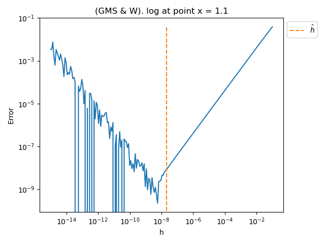
log
Step h* = 2.148e-08 using 3 iterations

problem = nd.SinProblem()
x = 1.0
kmin = 1.0e-15
kmax = 1.0e-1
step_array = np.logspace(-15.0, -1.0, number_of_points)
plot_error_vs_h_benchmark(problem, x, step_array, kmin, kmax)

problem = nd.SquareRootProblem()
x = 1.0
kmin = 1.0e-15
kmax = 1.0e-1
step_array = np.logspace(-15.0, -1.0, number_of_points)
plot_error_vs_h_benchmark(problem, x, step_array, kmin, kmax, relative_precision, True)

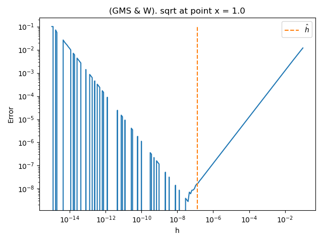
sqrt
Step h* = 1.264e-07 using 2 iterations

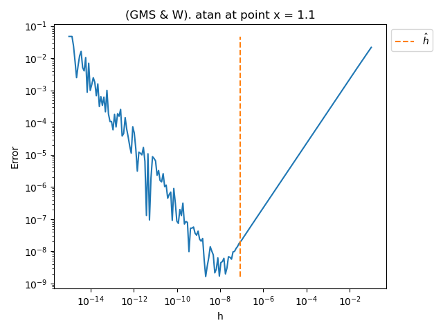
problem = nd.AtanProblem()
x = 1.1
kmin = 1.0e-15
kmax = 1.0e-1
step_array = np.logspace(-15.0, -1.0, number_of_points)
plot_error_vs_h_benchmark(problem, x, step_array, kmin, kmax)

See the history of steps during the bissection search

In G, M, S & W's method, the bisection algorithm produces a sequence of steps \((k_i)_{1 \leq i \leq n_{iter}}\) where \(n_{iter} \in \mathbb{N}\) is the number of iterations. These steps are meant to converge to an approximately optimal step of for the central finite difference formula of the second derivative. The optimal step \(k^\star\) for the central finite difference formula of the second derivative can be computed depending on the fourth derivative of the function. In the next example, we want to compute the absolute error between each intermediate step \(k_i\) and the exact value \(k^\star\) to see how close the algorithm gets to the exact step. The list of intermediate steps during the algorithm can be obtained thanks to the get_step_history() method.

In the next example, we print the intermediate steps k during the bissection algorithm that searches for a step such that the L ratio is satisfactory. The algorithm has two different methods to update the step:

• using the mean,

• using the mean in the logarithm space (this is generally much faster).

def plot_GMSW_step_history(problem, kmin, kmax, logscale):
    function = problem.get_function()
    name = problem.get_name()
    x = problem.get_x()
    algorithm = nd.GillMurraySaundersWright(function, x, verbose=True)
    step, number_of_iterations = algorithm.find_step(
        kmin=kmin, kmax=kmax, logscale=logscale
    )
    step_k_history = algorithm.get_step_history()
    print(f"Number of iterations = {number_of_iterations}")
    print(f"History of steps k : {step_k_history}")
    last_step_k = step_k_history[-1]
    print(f"Last step k : {last_step_k}")

    # Then we compute the exact step, using :meth:`~numericalderivative.SecondDerivativeCentral.compute_step`.
    fourth_derivative = problem.get_fourth_derivative()
    fourth_derivative_value = fourth_derivative(x)
    print(f"f^(4)(x) = {fourth_derivative_value}")
    absolute_precision = 1.0e-16
    exact_step_k, absolute_error = nd.SecondDerivativeCentral.compute_step(
        fourth_derivative_value, absolute_precision
    )
    print(f"Optimal step k for f^(2)(x) = {exact_step_k}")

    # Plot the absolute error between the exact step k and the intermediate k
    # of the algorithm.
    error_step_k = [
        abs(step_k_history[i] - exact_step_k) for i in range(len(step_k_history))
    ]
    fig = pl.figure()
    pl.title(f"GMSW on {name} at x = {x}. Log scale = {logscale}")
    pl.plot(range(len(step_k_history)), error_step_k, "o-")
    pl.xlabel("Iterations")
    pl.ylabel(r"$|k_i - k^\star|$")
    pl.yscale("log")
    ax = fig.gca()
    ax.xaxis.set_major_locator(MaxNLocator(integer=True))
    pl.tight_layout()

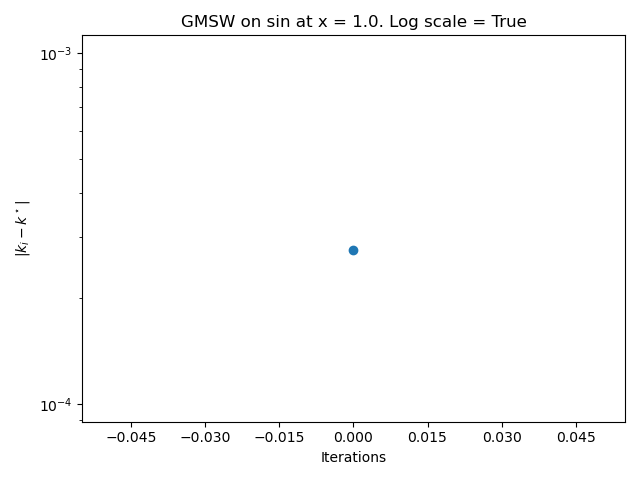
First, test the logarithmic log scale.

problem = nd.SinProblem()
kmin = 1.0e-15
kmax = 1.0e3
logscale = True
plot_GMSW_step_history(problem, kmin, kmax, logscale)

kmin = 1.000e-15, c(kmin) = inf
kmax = 1.000e+03, c(kmax) = 5.431e-15
Iter #0, kmin = 1.000e-15, kmax = 1.000e+03, k = 1.000e-06, c(k) = 4.753e-03
  c in [0.001, 0.1]: stop!
Number of iterations = 0
History of steps k : [np.float64(1.0000000000000004e-06)]
Last step k : 1.0000000000000004e-06
f^(4)(x) = 0.8414709848078965
Optimal step k for f^(2)(x) = 0.0002748213843759035

The previous figure shows that the algorithm does not necessarily reduce the distance to the optimal step when we use the logarithmic scale. The algorithm quickly stops and gets an error approximately equal to \(10^{-4}\).

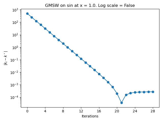
Secondly, test the ordinary scale, using the mean.

problem = nd.SinProblem()
kmin = 1.0e-15
kmax = 1.0e3
logscale = False
plot_GMSW_step_history(problem, kmin, kmax, logscale)

kmin = 1.000e-15, c(kmin) = inf
kmax = 1.000e+03, c(kmax) = 5.431e-15
Iter #0, kmin = 1.000e-15, kmax = 1.000e+03, k = 5.000e+02, c(k) = 1.262e-15
  c(k) < c_threshold_min: reduce kmax.
Iter #1, kmin = 1.000e-15, kmax = 5.000e+02, k = 2.500e+02, c(k) = 3.131e-15
  c(k) < c_threshold_min: reduce kmax.
Iter #2, kmin = 1.000e-15, kmax = 2.500e+02, k = 1.250e+02, c(k) = 1.120e-14
  c(k) < c_threshold_min: reduce kmax.
Iter #3, kmin = 1.000e-15, kmax = 1.250e+02, k = 6.250e+01, c(k) = 4.356e-14
  c(k) < c_threshold_min: reduce kmax.
Iter #4, kmin = 1.000e-15, kmax = 6.250e+01, k = 3.125e+01, c(k) = 1.731e-13
  c(k) < c_threshold_min: reduce kmax.
Iter #5, kmin = 1.000e-15, kmax = 3.125e+01, k = 1.562e+01, c(k) = 1.190e-15
  c(k) < c_threshold_min: reduce kmax.
Iter #6, kmin = 1.000e-15, kmax = 1.562e+01, k = 7.813e+00, c(k) = 2.480e-15
  c(k) < c_threshold_min: reduce kmax.
Iter #7, kmin = 1.000e-15, kmax = 7.813e+00, k = 3.906e+00, c(k) = 1.381e-15
  c(k) < c_threshold_min: reduce kmax.
Iter #8, kmin = 1.000e-15, kmax = 3.906e+00, k = 1.953e+00, c(k) = 1.731e-15
  c(k) < c_threshold_min: reduce kmax.
Iter #9, kmin = 1.000e-15, kmax = 1.953e+00, k = 9.766e-01, c(k) = 5.400e-15
  c(k) < c_threshold_min: reduce kmax.
Iter #10, kmin = 1.000e-15, kmax = 9.766e-01, k = 4.883e-01, c(k) = 2.034e-14
  c(k) < c_threshold_min: reduce kmax.
Iter #11, kmin = 1.000e-15, kmax = 4.883e-01, k = 2.441e-01, c(k) = 8.015e-14
  c(k) < c_threshold_min: reduce kmax.
Iter #12, kmin = 1.000e-15, kmax = 2.441e-01, k = 1.221e-01, c(k) = 3.194e-13
  c(k) < c_threshold_min: reduce kmax.
Iter #13, kmin = 1.000e-15, kmax = 1.221e-01, k = 6.104e-02, c(k) = 1.276e-12
  c(k) < c_threshold_min: reduce kmax.
Iter #14, kmin = 1.000e-15, kmax = 6.104e-02, k = 3.052e-02, c(k) = 5.105e-12
  c(k) < c_threshold_min: reduce kmax.
Iter #15, kmin = 1.000e-15, kmax = 3.052e-02, k = 1.526e-02, c(k) = 2.042e-11
  c(k) < c_threshold_min: reduce kmax.
Iter #16, kmin = 1.000e-15, kmax = 1.526e-02, k = 7.629e-03, c(k) = 8.167e-11
  c(k) < c_threshold_min: reduce kmax.
Iter #17, kmin = 1.000e-15, kmax = 7.629e-03, k = 3.815e-03, c(k) = 3.267e-10
  c(k) < c_threshold_min: reduce kmax.
Iter #18, kmin = 1.000e-15, kmax = 3.815e-03, k = 1.907e-03, c(k) = 1.307e-09
  c(k) < c_threshold_min: reduce kmax.
Iter #19, kmin = 1.000e-15, kmax = 1.907e-03, k = 9.537e-04, c(k) = 5.227e-09
  c(k) < c_threshold_min: reduce kmax.
Iter #20, kmin = 1.000e-15, kmax = 9.537e-04, k = 4.768e-04, c(k) = 2.091e-08
  c(k) < c_threshold_min: reduce kmax.
Iter #21, kmin = 1.000e-15, kmax = 4.768e-04, k = 2.384e-04, c(k) = 8.363e-08
  c(k) < c_threshold_min: reduce kmax.
Iter #22, kmin = 1.000e-15, kmax = 2.384e-04, k = 1.192e-04, c(k) = 3.345e-07
  c(k) < c_threshold_min: reduce kmax.
Iter #23, kmin = 1.000e-15, kmax = 1.192e-04, k = 5.960e-05, c(k) = 1.338e-06
  c(k) < c_threshold_min: reduce kmax.
Iter #24, kmin = 1.000e-15, kmax = 5.960e-05, k = 2.980e-05, c(k) = 5.352e-06
  c(k) < c_threshold_min: reduce kmax.
Iter #25, kmin = 1.000e-15, kmax = 2.980e-05, k = 1.490e-05, c(k) = 2.141e-05
  c(k) < c_threshold_min: reduce kmax.
Iter #26, kmin = 1.000e-15, kmax = 1.490e-05, k = 7.451e-06, c(k) = 8.563e-05
  c(k) < c_threshold_min: reduce kmax.
Iter #27, kmin = 1.000e-15, kmax = 7.451e-06, k = 3.725e-06, c(k) = 3.425e-04
  c(k) < c_threshold_min: reduce kmax.
Iter #28, kmin = 1.000e-15, kmax = 3.725e-06, k = 1.863e-06, c(k) = 1.370e-03
  c in [0.001, 0.1]: stop!
Number of iterations = 28
History of steps k : [500.0, 250.0, 125.0, 62.5, 31.25, 15.625, 7.812500000000001, 3.906250000000001, 1.9531250000000009, 0.976562500000001, 0.488281250000001, 0.244140625000001, 0.122070312500001, 0.061035156250001, 0.030517578125001, 0.015258789062501, 0.007629394531250999, 0.0038146972656259996, 0.0019073486328134999, 0.00095367431640725, 0.00047683715820412496, 0.0002384185791025625, 0.00011920928955178124, 5.960464477639062e-05, 2.980232238869531e-05, 1.4901161194847655e-05, 7.450580597923828e-06, 3.725290299461914e-06, 1.862645150230957e-06]
Last step k : 1.862645150230957e-06
f^(4)(x) = 0.8414709848078965
Optimal step k for f^(2)(x) = 0.0002748213843759035

In the previous plot, we see that the error first decreases down to an error approximately equal to \(10^{-4}\). Then the error slightly increases before the algorithm stops.